From Raw Reads to GWAS-Ready Data

A hands-on, HPC-native pipeline for WGS/WES processing, harmonization, and GWAS prep — no GCP, no Docker

The full command-line path from raw FASTQ to a GWAS-ready matrix – alignment, variant calling, joint genotyping, harmonization, phasing, imputation, and association testing, runnable on a laptop VM now and identically on real HPC later.

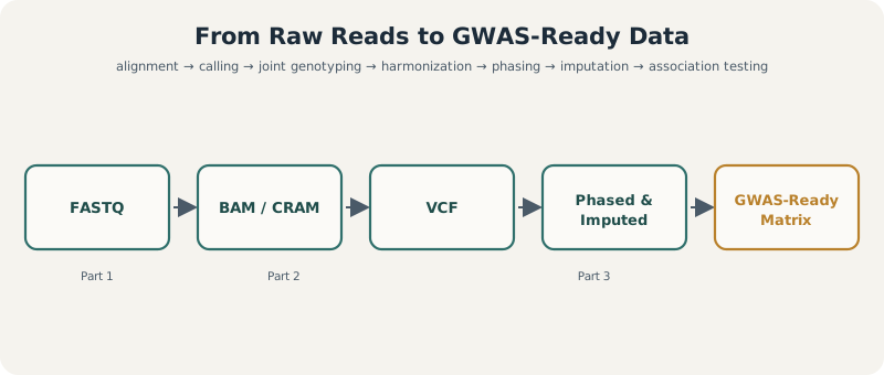
The full path this tutorial walks, end to end: every stage below is a real, copy-pasteable command, from a sequencer’s raw output to a matrix ready for association testing.

GATK PLINK Regenie HPC

How to use this

Each numbered step has a “What’s happening” explanation before the commands — read that first, then run the commands, then move on. No need to rush any of it. The tutorial is written for: - Part -1: environment setup on an Apple Silicon Mac (Lima Linux VM), since Linux-native bioinformatics tools don’t run natively on macOS ARM64 - Part 0: reference data staging, done once - Parts 1-3: the pipeline itself, runnable on your Mac at chr20/small-cohort scale now, and identically on real HPC later (just swap out the setup — every downstream command is the same either way)

Assume once you’re set up: - Reference: GRCh38 (Homo_sapiens_assembly38.fasta), matching known-sites VCFs from GATK resource bundle - Conda/mamba environments per tool group, to avoid dependency conflicts (set up in Part -1) - Everything here is designed to scale from “one trio on a laptop” to “thousands of WGS samples on a cluster” — the commands don’t change, only whether you prefix them with sbatch

---

Part -1 — Setting up your environment (Apple Silicon Mac, step by step)

What’s happening here, conceptually first: almost every tool in this pipeline (GATK, bwa-mem2, samtools, plink) was built and tested for Linux. macOS is Unix-like but not Linux — different system libraries, different binary format. On Intel Macs this mostly didn’t matter because the CPU instruction set matched Linux x86_64 builds. On Apple Silicon (M-series), the CPU architecture itself (ARM64) is different, so pre-built Linux binaries won’t run at all, and macOS-native ARM64 builds of these tools are incomplete or missing on bioconda. The fix is to run a real Linux virtual machine on your Mac — not emulation of individual programs, but an actual Linux kernel and userspace — so every tool installs and runs exactly as it would on your future HPC. This also means everything you learn about the environment transfers directly.

Step 1: Install Lima (the VM manager)

# Homebrew is macOS's package manager — if you don't have it:
/bin/bash -c "$(curl -fsSL https://raw.githubusercontent.com/Homebrew/install/HEAD/install.sh)"

# Lima runs a lightweight Linux VM with automatic file-sharing back to macOS
brew install lima

What this does: Lima creates a small Linux VM (using Apple’s native vz virtualization framework on M-series, so it’s fast — not slow software emulation) and automatically mounts your home directory inside it, so files you create feel local either way.

Step 2: Start a Linux VM sized for this work

limactl start --cpus 12 --memory 32 --disk 150 --arch aarch64 --vm-type vz default

What each flag does: - --cpus 12 — give the VM 12 of your performance cores; leaves headroom for macOS itself - --memory 32 — 32GB to the VM out of your 48GB total; leaves the rest for macOS + any GUI tools you’re running alongside - --disk 150 — reference genomes, VCFs, and intermediate BAMs eat disk fast; 150GB is a safe starting allocation for chr20-scale work (you’ll want more for full-genome runs) - --arch aarch64 — native ARM64 Linux, matching your M5 Pro’s actual architecture (no translation layer) - --vm-type vz — Apple’s native virtualization (faster than the older QEMU-based default on Apple Silicon)

# Drop into a shell inside the VM — this is now a real Linux machine
limactl shell default

Everything from here on runs inside this Lima shell, not in your normal macOS terminal. Your prompt will change to reflect this. To leave, just exit; to come back later, limactl start default (if stopped) then limactl shell default again.

Step 3: Install Miniforge/mamba inside the VM

What’s happening: conda/mamba is a package + environment manager built specifically for scientific software — it resolves complex dependency chains (a specific version of GATK needing a specific Java version needing specific system libraries) that would be painful to install by hand. mamba is a faster drop-in replacement for conda’s solver. We install it fresh inside the Linux VM (not on macOS) since that’s where all the Linux binaries will actually run.

curl -L -O "https://github.com/conda-forge/miniforge/releases/latest/download/Miniforge3-Linux-aarch64.sh"
bash Miniforge3-Linux-aarch64.sh -b -p $HOME/miniforge3
source $HOME/miniforge3/bin/activate
conda init bash
# close and reopen the Lima shell (or `source ~/.bashrc`) for this to take effect

Step 4: Create isolated environments per tool group

What’s happening: different bioinformatics tools sometimes need conflicting versions of shared libraries (e.g. different Python or htslib versions). Rather than fighting version conflicts in one giant environment, we create separate named environments — one activated at a time — so each tool group gets exactly the dependencies it wants without breaking another.

mamba create -n ngs-core -c bioconda -c conda-forge \
  fastp fastqc multiqc bwa-mem2 samtools sambamba gatk4 bcftools \
  vcftools plink plink2 mosdepth -y

mamba create -n ngs-sv -c bioconda manta smoove truvari -y

mamba create -n ngs-phase -c bioconda shapeit4 beagle eagle -y

mamba create -n ngs-gwas -c bioconda -c conda-forge regenie -y

Why split this way: ngs-core covers Part 1 + most of Part 2 (alignment, calling, basic QC). ngs-sv isolates the structural-variant callers, which sometimes pin older/different library versions. ngs-phase and ngs-gwas isolate the Part 3 tools similarly. You’ll conda activate ngs-core (etc.) before running the relevant commands — one environment active at a time.

Before trusting any of this, verify the key tools actually resolved to working binaries (aarch64 bioconda coverage isn’t 100% for every package):

conda activate ngs-core
bwa-mem2 version
gatk --version
samtools --version

If any of these fail to install or run, the fallback is forcing that specific package through the linux-64 (Intel Linux) channel, which the VM’s Linux kernel can still execute via qemu-user-static emulation — slower for that one tool, but everything else stays native:

mamba create -n ngs-core-x64 --platform linux-64 -c bioconda -c conda-forge <tool-that-failed> -y

Step 5: Confirm your resource allocation matches what you planned

nproc                # should show 12 (or whatever you allocated)
free -h              # should show ~32GB total
df -h $HOME          # confirm your disk allocation

Step 6: A sane working directory layout

What’s happening: genomics pipelines generate a lot of intermediate files (raw reads → trimmed reads → BAM → dedup BAM → recalibrated BAM → GVCF → joint VCF → filtered VCF → phased VCF → imputed VCF, per sample, per chromosome). Without a deliberate layout you will lose track of what’s what within a day. This structure mirrors what you’ll see on real HPC filesystems.

mkdir -p ~/ngs_work/{refs,raw,work/{trimmed,aligned,dedup,bqsr,gvcf,joint,filtered,phased,imputed},qc,scripts}
cd ~/ngs_work

From here, Part 0 (reference staging) and Part 1 onward all run inside this Lima Linux shell, with ngs-core (or the relevant environment) activated.

---

Part 0 — Staging reference data (run once, reuse across all samples)

What’s happening: every downstream step needs a common coordinate system to align reads to and a set of “known truth” variant sites to calibrate against. This section downloads exactly those shared resources once, so every sample you process afterward references the identical files — consistency here is what makes results comparable across samples and, eventually, across collaborating cohorts like FinnGen partners.

mkdir -p refs/{genome,vqsr,phasing,giab}
cd refs

# --- GRCh38 reference + GATK resource bundle (public, no GCP account required) ---
gsutil -m cp gs://gcp-public-data--broad-references/hg38/v0/Homo_sapiens_assembly38.fasta \
  gs://gcp-public-data--broad-references/hg38/v0/Homo_sapiens_assembly38.fasta.fai \
  gs://gcp-public-data--broad-references/hg38/v0/Homo_sapiens_assembly38.dict \
  genome/

gsutil -m cp \
  gs://gcp-public-data--broad-references/hg38/v0/Homo_sapiens_assembly38.dbsnp138.vcf.gz \
  gs://gcp-public-data--broad-references/hg38/v0/Homo_sapiens_assembly38.dbsnp138.vcf.gz.tbi \
  gs://gcp-public-data--broad-references/hg38/v0/Mills_and_1000G_gold_standard.indels.hg38.vcf.gz \
  gs://gcp-public-data--broad-references/hg38/v0/Mills_and_1000G_gold_standard.indels.hg38.vcf.gz.tbi \
  gs://gcp-public-data--broad-references/hg38/v0/Homo_sapiens_assembly38.known_indels.vcf.gz \
  gs://gcp-public-data--broad-references/hg38/v0/Homo_sapiens_assembly38.known_indels.vcf.gz.tbi \
  vqsr/

# --- VQSR training/truth resources ---
gsutil -m cp \
  gs://gcp-public-data--broad-references/hg38/v0/hapmap_3.3.hg38.vcf.gz \
  gs://gcp-public-data--broad-references/hg38/v0/1000G_omni2.5.hg38.vcf.gz \
  gs://gcp-public-data--broad-references/hg38/v0/1000G_phase1.snps.hg38.vcf.gz \
  vqsr/

# --- Index BWA-MEM2 reference (do this once, it's slow) ---
bwa-mem2 index genome/Homo_sapiens_assembly38.fasta

# --- 1000 Genomes high-coverage phased panel (for SHAPEIT4/Eagle/Beagle) ---
for chr in $(seq 1 22); do
  wget -P phasing/ \
    "http://ftp.1000genomes.ebi.ac.uk/vol1/ftp/data_collections/1000G_2504_high_coverage/working/20220422_3202_phased_SNV_INDEL_SV/1kGP_high_coverage_Illumina.chr${chr}.filtered.SNV_INDEL_SV_phased_panel.vcf.gz"
done

# --- Genetic maps (Beagle/Eagle format, GRCh38) ---
wget -P phasing/ https://bochet.gcc.biostat.washington.edu/beagle/genetic_maps/plink.GRCh38.map.zip
unzip phasing/plink.GRCh38.map.zip -d phasing/

# --- GIAB truth set (HG002) for validating your pipeline against known-truth calls ---
# Browse the current directory tree first — URL paths shift periodically:
# https://ftp-trace.ncbi.nlm.nih.gov/ReferenceSamples/giab/
# Grab the GRCh38-aligned AJ-trio (HG002/3/4) FASTQ or CRAM set from there.

# --- Sanity checksum everything before trusting it ---
find . -type f \( -name "*.vcf.gz" -o -name "*.fasta" \) -exec md5sum {} \; > checksums.txt

If gsutil isn’t available on your HPC (common — many clusters block outbound GCS auth), use the plain HTTPS mirror instead: prefix each path with https://storage.googleapis.com/gcp-public-data--broad-references/... and swap gsutil -m cp for wget.

What each of these files is actually for, since it matters later when something goes wrong: - Homo_sapiens_assembly38.fasta (+.fai/.dict) — the coordinate system itself. Every position you’ll ever report (“chr20:1234567”) is only meaningful relative to this exact file. Mixing reference builds (GRCh37 vs GRCh38) between steps is one of the most common and hardest-to-notice pipeline bugs. - dbsnp138.vcf.gz — a catalog of previously observed variant positions, used to annotate/flag known vs novel sites and as a training resource - Mills...indels and known_indels — curated “trustworthy” indel sites, used specifically by BQSR to know which mismatches are real biology (leave alone) vs sequencing error (recalibrate away) - hapmap, 1000G_omni2.5, 1000G_phase1.snps — high-confidence SNP truth sets used later by VQSR to learn what a real variant’s statistical signature looks like, versus an artifact’s - the 1000G phased panel + genetic maps — used in Part 3 for phasing and imputation, which need a large reference cohort’s known haplotype structure to infer missing/uncertain genotypes in your own samples - GIAB HG002 — the one sample in this whole tutorial where you actually know the right answer, which is why it’s used for validation exercises later

---

PART 1 — Raw FASTQ → Analysis-Ready BAM/CRAM

1.1 Sanity-check and QC raw reads

What’s happening: a sequencer doesn’t output “the genome” — it outputs millions of short, overlapping, imperfect text reads (FASTQ format: a DNA sequence + a per-base quality score for each read). Before you spend hours aligning bad data, you check whether the raw reads themselves are trustworthy: are quality scores dropping off, is there leftover adapter sequence the sequencer failed to strip, is the GC content distribution what you’d expect from human DNA (a skew can mean contamination). fastp then actively cleans the reads — trimming adapters and low-quality bases — before anything touches the reference genome.

# Per-sample QC
fastqc sample_R1.fastq.gz sample_R2.fastq.gz -o qc/ -t 8

# Adapter trimming + quality filtering + auto-detection of adapters (fastp is faster than trimmomatic and gives a JSON report)
fastp \
  -i sample_R1.fastq.gz -I sample_R2.fastq.gz \
  -o trimmed_R1.fastq.gz -O trimmed_R2.fastq.gz \
  --detect_adapter_for_pe \
  --qualified_quality_phred 20 \
  --length_required 36 \
  --thread 8 \
  --json fastp_sample.json --html fastp_sample.html

# Aggregate QC across a whole batch — this is what you'll actually eyeball daily
multiqc qc/ fastp_*.json -o multiqc_report/

What to flag before proceeding: per-base quality drop-off, adapter content >5%, GC content bimodality (contamination), duplication rate pre-alignment (library complexity proxy).

1.2 Alignment (BWA-MEM2 — faster drop-in replacement for BWA-MEM, same output)

What’s happening: alignment is the step where each of those millions of short reads gets placed at its most likely position of origin on the reference genome. bwa-mem2 does this using an FM-index (a compressed, searchable representation of the whole genome built by bwa-mem2 index) to rapidly find candidate matching regions, then does a proper local alignment (allowing for mismatches/small indels from real biological variation or sequencing error) to pick the best position and produce a CIGAR string describing exactly how the read lines up. The output SAM/BAM format is essentially “for every read: where it landed, how well it matched, and how confident we are.” The read group (-R string) isn’t decoration — it’s metadata GATK relies on downstream to know which reads came from the same physical sequencing run, which matters for error-model calibration in BQSR and for correctly attributing genotypes to the right sample.

# Index reference once
bwa-mem2 index Homo_sapiens_assembly38.fasta

# Align with proper read group (mandatory for GATK downstream — get this wrong and BQSR/HaplotypeCaller will silently misbehave)
bwa-mem2 mem -t 16 \
  -R "@RG\tID:sample1_L001\tSM:sample1\tPL:ILLUMINA\tLB:lib1\tPU:flowcell1.lane1" \
  Homo_sapiens_assembly38.fasta \
  trimmed_R1.fastq.gz trimmed_R2.fastq.gz \
  | samtools sort -@ 8 -o sample1.sorted.bam -
samtools index sample1.sorted.bam

For multi-lane samples, align each lane separately with distinct ID/PU, same SM, then merge:

samtools merge -@ 8 sample1.merged.bam sample1_L001.sorted.bam sample1_L002.sorted.bam
samtools index sample1.merged.bam

1.3 Mark duplicates

What’s happening: PCR amplification during library prep, and sometimes the sequencer itself (optical duplicates), can produce multiple reads that are actually copies of the exact same original DNA fragment rather than independent observations. If you count these as independent evidence, you’ll inflate confidence in variant calls that are really just one PCR-duplicated read counted five times. This step doesn’t delete duplicates — it flags them (a SAM flag bit) so downstream tools like HaplotypeCaller know to down-weight or ignore them, while the raw data is preserved for auditing.

# GATK's MarkDuplicatesSpark parallelizes well; sambamba markdup is a lighter/faster alternative for large WGS batches
gatk MarkDuplicatesSpark \
  -I sample1.merged.bam \
  -O sample1.dedup.bam \
  -M sample1.dedup_metrics.txt \
  --spark-master local[16]

# Alternative (often faster at scale):
sambamba markdup -t 16 sample1.merged.bam sample1.dedup.bam

1.4 Base Quality Score Recalibration (BQSR)

What’s happening: the sequencer’s own per-base quality scores are a machine’s estimate of its own error rate, and that estimate is systematically biased in predictable ways — by position in the read, by the specific sequence context, by which machine cycle produced the base. BQSR builds an empirical error model by comparing observed mismatches against the known truth sites (dbSNP/Mills/known indels you staged in Part 0) — any mismatch at a known-variant site is assumed to be real biology, while mismatches everywhere else are assumed to be sequencing error, and the model learns the actual error rate per context. ApplyBQSR then rewrites each base’s quality score using this corrected model. Downstream variant callers weight evidence by these quality scores directly, so this step measurably improves variant calling accuracy — it’s not cosmetic.

gatk BaseRecalibrator \
  -I sample1.dedup.bam \
  -R Homo_sapiens_assembly38.fasta \
  --known-sites Homo_sapiens_assembly38.dbsnp138.vcf.gz \
  --known-sites Mills_and_1000G_gold_standard.indels.hg38.vcf.gz \
  --known-sites Homo_sapiens_assembly38.known_indels.vcf.gz \
  -O sample1.recal.table

gatk ApplyBQSR \
  -I sample1.dedup.bam \
  -R Homo_sapiens_assembly38.fasta \
  --bqsr-recal-file sample1.recal.table \
  -O sample1.final.bam

1.5 Convert to CRAM (mandatory at scale — ~40-60% smaller than BAM, and this matters a lot once you’re storing thousands of WGS samples)

What’s happening: BAM stores every read’s full sequence even though most of it matches the reference exactly. CRAM instead stores only the differences from the reference (which you supply via -T) plus a reference-independent fallback for unmapped/unusual reads, then compresses that much smaller representation further. The tradeoff is that a CRAM file is meaningless without the exact reference FASTA that produced it — which is exactly why Part 0 pinned one canonical reference file for the whole pipeline.

samtools view -T Homo_sapiens_assembly38.fasta -C -@ 8 \
  -o sample1.final.cram sample1.final.bam
samtools index sample1.final.cram

1.6 Post-alignment QC gates — run these before anyone trusts the sample

What’s happening: this is the checkpoint where you decide, quantitatively, whether a sample is good enough to keep processing or needs to be flagged/excluded/re-sequenced. Each metric answers a distinct question: coverage/depth (samtools coverage, mosdepth) — did we sequence deeply enough at each position to call genotypes confidently, and are there suspicious dropouts that might indicate a deletion or a capture failure; samtools stats/flagstat — did alignment itself go well (mapping rate, proper pairing, insert size distribution matching the library prep expectation); contamination (VerifyBamID2) — is this BAM secretly a mixture of two individuals’ DNA (a real risk in any wet-lab pipeline, from sample swaps to cross-contamination), measured by checking whether allele frequencies at known-variant sites look like they came from one clean genome or a mixture.

# Coverage / depth
samtools coverage sample1.final.cram > sample1.coverage.txt
mosdepth --by 500 sample1 sample1.final.cram   # fast, windowed depth — great for spotting CNV-scale dropouts

# Insert size, alignment stats
samtools stats sample1.final.cram > sample1.stats.txt
samtools flagstat sample1.final.cram > sample1.flagstat.txt

# Contamination check (critical for WGS/WES QC gates — cross-sample or cross-species contamination)
gatk CollectFingerprintingDetailMetrics \
  -I sample1.final.cram -R Homo_sapiens_assembly38.fasta \
  -O sample1.fingerprint --HAPLOTYPE_MAP hapmap_3.3.hg38.map

VerifyBamID2 --SVDPrefix resource/1000g.phase3 \
  --Reference Homo_sapiens_assembly38.fasta --BamFile sample1.final.cram

Standard gate thresholds to codify into a QC pipeline: mean coverage (≥30x WGS / ≥50-100x on-target WES), %reads mapped ≥95%, duplication rate <20%, contamination (FREEMIX) <3%, sex-check concordance (via chrX/Y coverage ratio) against reported sex.

---

PART 2 — Variant Calling, Joint Genotyping, SV Calling, and VCF-Level QC

2.1 Per-sample GVCF calling (GATK’s scalable design — call once per sample, joint-genotype later without re-calling)

What’s happening: HaplotypeCaller doesn’t just look at one position at a time — it locally reassembles the reads in each region into candidate haplotypes (via a local de Bruijn-like graph), then uses a statistical model to score how well each candidate haplotype explains the observed reads, which is what lets it call indels accurately and not just simple substitutions. Critically, we run it in GVCF mode (-ERC GVCF), which records a confidence estimate at every position — including ones with no variant — rather than only variant sites. This is the design that makes cohort-scale calling tractable: if you called each sample against a fixed set of “known” variant sites, you’d never discover a variant that’s rare or private to your cohort; GVCF mode defers the “is this actually a variant across the cohort” decision to the joint-genotyping step next, while still only running the expensive per-read reassembly once per sample.

gatk HaplotypeCaller \
  -I sample1.final.cram \
  -R Homo_sapiens_assembly38.fasta \
  -O sample1.g.vcf.gz \
  -ERC GVCF \
  --native-pair-hmm-threads 8

For WES, restrict to the capture region:

gatk HaplotypeCaller \
  -I sample1.final.cram -R Homo_sapiens_assembly38.fasta \
  -L capture_targets.interval_list -ip 100 \
  -O sample1.g.vcf.gz -ERC GVCF

2.2 Joint genotyping across a cohort (this is where FinnGen-scale joint calling happens)

What’s happening: GenomicsDBImport merges each sample’s per-position confidence records (from the GVCFs) into an efficient, queryable on-disk database — think of it as a sparse matrix of “sample × genomic position → evidence,” built specifically so it scales to thousands of samples without exploding in size or IO cost, which flat CombineGVCFs doesn’t do well past a few hundred samples. GenotypeGVCFs then makes the actual joint calling decision: at every position where any sample showed evidence of a variant, it looks across all samples simultaneously to decide the final genotype for each individual — a site that looked marginal in one sample alone can become a confident call once you see the same allele recurring across the cohort, which is exactly the statistical leverage joint calling gives you over calling each sample in isolation.

# Consolidate GVCFs — GenomicsDBImport scales far better than CombineGVCFs for thousands of samples
gatk GenomicsDBImport \
  --genomicsdb-workspace-path cohort_db_chr1 \
  -L chr1 \
  --sample-name-map cohort.sample_map.txt \
  --batch-size 50 \
  --reader-threads 8

# sample_map.txt format: sample_id<TAB>path/to/sample.g.vcf.gz  (one per line)

gatk GenotypeGVCFs \
  -R Homo_sapiens_assembly38.fasta \
  -V gendb://cohort_db_chr1 \
  -O cohort_chr1.vcf.gz

Run per-chromosome in parallel across the cluster, then merge:

bcftools concat -Oz -o cohort.joint.vcf.gz cohort_chr*.vcf.gz
bcftools index -t cohort.joint.vcf.gz

2.3 Variant Quality Score Recalibration (VQSR) — the actual filtering step that matters most for downstream GWAS validity

What’s happening: raw joint-called variants include real biology and a substantial number of technical artifacts (mapping errors, systematic sequencing biases, assembly mistakes in repetitive regions). A single hard threshold on any one annotation (e.g. “reject anything with QD < 2”) is crude because artifacts don’t look identical across the genome. VQSR instead trains a Gaussian mixture model on several per-variant annotations simultaneously (QD = quality normalized by depth, MQ = mapping quality, FS/SOR = strand bias measures, ReadPosRankSum = whether the variant allele clusters suspiciously at read ends) using the truth/training sites from Part 0 as positive examples of “this is what real variants look like.” Every variant in your callset then gets a score for how well it resembles the truth-set variants’ statistical fingerprint, and ApplyVQSR cuts at a sensitivity threshold (e.g. 99.5% — “keep the score cutoff that retains 99.5% of the training truth sites”) rather than an arbitrary single-metric threshold. This is genuinely more powerful than hard filtering because it learns the joint distribution of what real variants look like across all metrics at once, not each metric independently.

# SNPs
gatk VariantRecalibrator \
  -R Homo_sapiens_assembly38.fasta -V cohort.joint.vcf.gz \
  --resource:hapmap,known=false,training=true,truth=true,prior=15.0 hapmap_3.3.hg38.vcf.gz \
  --resource:omni,known=false,training=true,truth=false,prior=12.0 1000G_omni2.5.hg38.vcf.gz \
  --resource:1000G,known=false,training=true,truth=false,prior=10.0 1000G_phase1.snps.hg38.vcf.gz \
  --resource:dbsnp,known=true,training=false,truth=false,prior=2.0 Homo_sapiens_assembly38.dbsnp138.vcf.gz \
  -an QD -an MQ -an MQRankSum -an ReadPosRankSum -an FS -an SOR \
  -mode SNP \
  -O cohort.snps.recal --tranches-file cohort.snps.tranches

gatk ApplyVQSR \
  -R Homo_sapiens_assembly38.fasta -V cohort.joint.vcf.gz \
  --recal-file cohort.snps.recal --tranches-file cohort.snps.tranches \
  --truth-sensitivity-filter-level 99.5 -mode SNP \
  -O cohort.snps.filtered.vcf.gz

# Indels (same pattern, different annotations/resources)
gatk VariantRecalibrator \
  -R Homo_sapiens_assembly38.fasta -V cohort.snps.filtered.vcf.gz \
  --resource:mills,known=false,training=true,truth=true,prior=12.0 Mills_and_1000G_gold_standard.indels.hg38.vcf.gz \
  --resource:dbsnp,known=true,training=false,truth=false,prior=2.0 Homo_sapiens_assembly38.dbsnp138.vcf.gz \
  -an QD -an FS -an ReadPosRankSum -an MQRankSum -an SOR \
  -mode INDEL -O cohort.indels.recal --tranches-file cohort.indels.tranches

gatk ApplyVQSR \
  -R Homo_sapiens_assembly38.fasta -V cohort.snps.filtered.vcf.gz \
  --recal-file cohort.indels.recal --tranches-file cohort.indels.tranches \
  --truth-sensitivity-filter-level 99.0 -mode INDEL \
  -O cohort.final.vcf.gz

For cohorts too small for reliable VQSR (roughly <30 samples), fall back to hard filtering with VariantFiltration using the same annotation thresholds as tranches approximate — worth knowing both paths since production cohorts often need to bootstrap from small pilot batches.

2.4 Structural variants (SNVs/indels are not the whole story — this is explicitly in scope per the JD)

What’s happening: HaplotypeCaller is built for small variants (SNVs and indels typically under ~50bp) because its local reassembly approach breaks down for larger rearrangements. Structural variants — deletions, duplications, insertions, inversions, translocations spanning hundreds to millions of bases — need different evidence entirely: read pairs whose insert size or orientation doesn’t match expectation, split reads that align partially to two different genomic locations, and coverage depth changes. Manta scans for exactly these signal types and assembles breakpoints from them; smoove (built on lumpy+svtyper+duphold) is a lighter, faster alternative tuned for running consistently across large cohorts, followed by a merge/genotype step so that an SV detected in one sample gets properly genotyped (present/absent/heterozygous) across every other sample in the cohort, the SV equivalent of joint genotyping in section 2.2.

# Manta — good general-purpose SV caller (deletions, duplications, insertions, inversions, translocations)
configManta.py --bam sample1.final.cram --referenceFasta Homo_sapiens_assembly38.fasta \
  --runDir manta_sample1
manta_sample1/runWorkflow.py -j 8

# smoove — lighter-weight, good for cohort-scale SV joint calling
smoove call --outdir sv_out/ --name sample1 --fasta Homo_sapiens_assembly38.fasta \
  --exclude exclude.cnvnator_100bp.GRCh38.20170403.bed -p 1 --genotype sample1.final.cram

smoove merge --name cohort --fasta Homo_sapiens_assembly38.fasta sv_out/*.genotyped.vcf.gz
smoove genotype -d -x -p 1 --name cohort-joint --outdir genotyped/ \
  --fasta Homo_sapiens_assembly38.fasta --vcf cohort.merged.sites.vcf.gz sample1.final.cram

2.5 VCF-level QC (bcftools + vcftools — the daily-driver tools for harmonization QC)

What’s happening: this is sample-level QC done after variant calling rather than on the raw reads — sometimes a sample only reveals a problem once you can see its genotypes in the context of the whole cohort. Per-sample missingness (how many sites failed to get a confident genotype call) flags samples with poor overall data quality. Heterozygosity rate is a classic contamination/inbreeding proxy — unusually high heterozygosity can indicate sample contamination (looks like a mixture of two genomes), unusually low can indicate inbreeding or a technical artifact. Ts/Tv ratio (transition vs transversion substitution rate) has a well-known expected value for real human variation (~2.0-2.1 genome-wide, ~3.0 in exomes) — a callset that deviates substantially is a signal something upstream (often VQSR filtering) went wrong. The KING kinship table detects unexpected relatedness or accidental sample duplicates before they contaminate GWAS results, since undetected relatedness violates the independence assumption most association tests rely on.

# Site-level metrics
bcftools stats cohort.final.vcf.gz > cohort.stats.txt

# Per-sample missingness, heterozygosity, Ts/Tv — classic sample-QC exclusion criteria
vcftools --gzvcf cohort.final.vcf.gz --missing-indv --out cohort_qc
vcftools --gzvcf cohort.final.vcf.gz --het --out cohort_qc
vcftools --gzvcf cohort.final.vcf.gz --TsTv-summary --out cohort_qc

# Relatedness / duplicate-sample detection — essential before any GWAS
plink2 --vcf cohort.final.vcf.gz --make-king-table --out cohort_king

---

PART 3 — Harmonization, Phasing, Imputation, and Building the GWAS-Ready Matrix

3.1 Normalize and harmonize variant representation (the step everyone underestimates — left-alignment/normalization mismatches silently break joint analyses across cohorts, e.g. FinnGen + external partners)

What’s happening: the same real-world variant can be written multiple equivalent ways in VCF format — a multi-allelic site (one position, several alternate alleles) can be listed as one record or split into several, and indels near repetitive sequence can be left-aligned differently depending on which tool produced the call. If two cohorts represent the identical variant differently, a naive position-based merge will treat them as two different variants and silently lose the overlap. bcftools norm -m -any splits multi-allelic sites into separate biallelic records and left-aligns indels against the reference to a single canonical representation, which is what makes downstream joins across samples, cohorts, and reference panels actually work. The chromosome-naming step handles the other classic mismatch — some tools/panels use chr1, others use 1 for the same chromosome, and a merge between mismatched naming conventions fails or silently drops everything.

bcftools norm -f Homo_sapiens_assembly38.fasta -m -any cohort.final.vcf.gz -Oz -o cohort.norm.vcf.gz
bcftools index -t cohort.norm.vcf.gz

# Harmonize chromosome naming (chr1 vs 1 — the single most common cross-cohort merge failure)
bcftools annotate --rename-chrs chr_name_conv.txt cohort.norm.vcf.gz -Oz -o cohort.harm.vcf.gz

3.2 Convert to PLINK format and apply standard GWAS-QC filters

What’s happening: PLINK’s binary format (.bed/.bim/.fam) is far more compact and faster to compute on than VCF for the kind of matrix-wide operations GWAS tools need, so this is the standard conversion point. The four filters here are the textbook GWAS quality gates, each guarding against a different failure mode: --geno 0.02 drops variants missing genotype calls in >2% of samples (usually a sign the site is technically unreliable, not biologically interesting); --mind 0.02 drops samples missing >2% of variants (a poor-quality sample, analogous to the per-sample missingness check in 2.5 but now enforced as a hard exclusion); --maf 0.01 drops variants below 1% minor allele frequency, since very rare variants have too little statistical power for standard GWAS and are also where genotyping/calling errors masquerade as “variants” most easily; --hwe 1e-6 flags departures from Hardy-Weinberg equilibrium, which in a large random-mating population is often a signal of genotyping error rather than real biology (true selection/population-structure departures exist but are rarer than artifacts at this threshold).

plink2 --vcf cohort.harm.vcf.gz --make-bed --out cohort_plink --set-all-var-ids @:#:\$r:\$a

plink2 --bfile cohort_plink \
  --geno 0.02 --mind 0.02 --maf 0.01 --hwe 1e-6 \
  --make-bed --out cohort_qc1

# LD-based pruning for PCA/kinship input
plink2 --bfile cohort_qc1 --indep-pairwise 200 50 0.2 --out prune
plink2 --bfile cohort_qc1 --extract prune.prune.in --make-bed --out cohort_pruned

3.3 Population structure and relatedness (needed both for QC exclusions and as GWAS covariates)

What’s happening: GWAS association tests assume, at minimum, that samples are unrelated and that allele frequency differences aren’t confounded with the trait through ancestry alone (population stratification — a classic false-positive source where an allele is just more common in one ancestral group that also happens to differ in the trait for unrelated cultural/environmental reasons). KING-robust kinship estimates relatedness directly from genotype sharing patterns in a way that’s robust even in the presence of population structure, letting you catch cryptic relatedness before it inflates your test statistics. PCA on the LD-pruned genotypes captures the main axes of ancestry-driven genetic variation in your cohort; the top PCs get included as covariates in the GWAS model in Part 3.7 specifically to soak up and control for that stratification signal.

# KING-robust kinship for relatedness/family structure — standard in FinnGen-style pipelines
plink2 --bfile cohort_pruned --make-king-table --out cohort_kinship

# PCA for ancestry / population-stratification covariates
plink2 --bfile cohort_pruned --pca 10 --out cohort_pca

3.4 Phasing (statistical, reference-based haplotype phasing — precursor to imputation)

What’s happening: standard genotyping tells you which two alleles a person carries at each position (e.g. heterozygous A/G) but not which chromosome copy each allele sits on — that’s phase, and imputation algorithms specifically need phased haplotypes to work (they extend known haplotype blocks, not independent genotypes). SHAPEIT4/Eagle2 solve this statistically: given your cohort’s genotypes plus a large reference panel of already-phased haplotypes (the 1000G panel from Part 0), they find the most probable haplotype assignment by looking for chunks of your sample’s genotype pattern that match known haplotype segments in the reference — real chromosomes are mosaics of a surprisingly limited number of ancestral haplotype blocks, which is exactly the structure phasing algorithms exploit.

# SHAPEIT4 — accurate and fast for large biobank-scale cohorts
shapeit4 --input cohort_qc1.chr20.vcf.gz \
  --map genetic_map_chr20.b38.txt \
  --region chr20 \
  --reference 1000GP.chr20.phased.vcf.gz \
  --output cohort.chr20.phased.vcf.gz \
  --thread 16

# Eagle2 is the common alternative, especially paired with Beagle/Minimac imputation pipelines
eagle --vcfRef 1000GP.chr20.bcf --vcfTarget cohort_qc1.chr20.vcf.gz \
  --geneticMapFile genetic_map_hg38.txt.gz \
  --outPrefix cohort.chr20.eagle_phased --numThreads 16

3.5 Imputation to a reference panel (Beagle5 shown; swap for Minimac4 if using the Michigan/TOPMed panel conventions)

What’s happening: your directly-called genotypes cover only the positions your sequencing/calling actually captured well. Imputation fills in genotypes at additional positions present in the (much larger, deeply-sequenced) reference panel, by matching your phased haplotype segments against the panel’s haplotypes and inferring which panel haplotype your sample most likely shares at each additional position — essentially borrowing statistical power from the reference panel’s depth to extend your effective variant coverage far beyond what you directly sequenced. Every imputed genotype comes with an uncertainty estimate (DR2/INFO score — how confidently the algorithm could make that inference), which is why the very next line filters on it: low-confidence imputed calls are worse than not having the variant at all, since they inject noise into a GWAS as if it were real signal.

java -Xmx32g -jar beagle.jar \
  gt=cohort.chr20.phased.vcf.gz \
  ref=1000GP.chr20.bref3 \
  map=plink.chr20.GRCh38.map \
  out=cohort.chr20.imputed \
  nthreads=16

# Post-imputation QC: filter on imputation INFO score — this threshold is a direct input to your downstream SBayesR/GCTB work
bcftools view -i 'INFO/DR2>0.8' cohort.chr20.imputed.vcf.gz -Oz -o cohort.chr20.imputed.qc.vcf.gz

3.6 Assemble the analysis-ready GWAS matrix

What’s happening: simple bookkeeping at this point — stitching the per-chromosome imputed files back into one genome-wide dataset and converting to PLINK2’s .pgen format, which stores dosages (fractional genotype probabilities from imputation, not just hard 0/1/2 calls) far more efficiently than VCF at cohort scale. The final MAF filter here is a second, post-imputation pass — imputation itself can introduce very-rare spurious variants at the edges of panel coverage, so re-applying a frequency floor right before association testing is standard practice.

# Concatenate imputed chromosomes, convert to PLINK2 pgen for efficient large-scale storage
bcftools concat -Oz -o cohort.imputed.allchr.vcf.gz cohort.chr*.imputed.qc.vcf.gz
plink2 --vcf cohort.imputed.allchr.vcf.gz --make-pgen --out cohort_gwas_ready

# Final MAF/INFO filters typically applied right before association testing
plink2 --pfile cohort_gwas_ready --maf 0.01 --make-pgen --out cohort_gwas_final

3.7 Run the GWAS (regenie — the standard for biobank-scale mixed-model GWAS; handles related individuals and population structure natively)

What’s happening: naive linear/logistic regression of trait-on-genotype, one variant at a time, breaks down at biobank scale because related individuals and residual population structure inflate false positives (the same confound PCA/kinship in 3.3 partially addresses, but not completely). Regenie’s two-step design handles this more robustly: Step 1 fits a whole-genome ridge regression using directly-genotyped variants to build a polygenic prediction of the trait per individual, which effectively captures and removes the confounding structure (relatedness + polygenic background) before any single-variant test happens. Step 2 then tests each imputed variant for association with the trait residual left after subtracting that Step-1 prediction — dramatically better calibrated than testing raw trait values directly, especially for related samples or rare-variant/case-control-imbalanced traits, which is why --firth (a bias-corrected logistic regression) is included for binary traits.

# Step 1: whole-genome ridge regression on genotyped (not imputed) variants
regenie --step 1 --bed cohort_qc1 \
  --phenoFile pheno.txt --covarFile covars_with_PCs.txt \
  --bsize 1000 --bt --out cohort_step1

# Step 2: association testing on imputed dosages
regenie --step 2 --pgen cohort_gwas_final \
  --phenoFile pheno.txt --covarFile covars_with_PCs.txt \
  --bsize 400 --bt --firth --approx \
  --pred cohort_step1_pred.list \
  --out cohort_gwas_results

3.8 Where GCTB/SBayesR picks up from here

The cohort_gwas_results summary statistics (chr, pos, effect allele, beta, se, p, N) plus an LD reference panel built from cohort_pruned (or a matched external panel) are exactly the two inputs your SBayesR workflow expects — same COJO-format conventions you’ve already worked through with GCTB. This is the natural handoff point from “production sequencing pipeline” into the polygenic-score/methods work mentioned as a growth area in the role.

---

Quick reference: end-to-end command chain (one sample, condensed)

fastp -i R1.fq.gz -I R2.fq.gz -o t1.fq.gz -O t2.fq.gz
bwa-mem2 mem -R "@RG\tID:s1\tSM:s1\tPL:ILLUMINA" ref.fa t1.fq.gz t2.fq.gz | samtools sort -o s1.bam -
gatk MarkDuplicatesSpark -I s1.bam -O s1.dedup.bam
gatk BaseRecalibrator -I s1.dedup.bam -R ref.fa --known-sites known.vcf.gz -O recal.table
gatk ApplyBQSR -I s1.dedup.bam -R ref.fa --bqsr-recal-file recal.table -O s1.final.bam
gatk HaplotypeCaller -I s1.final.bam -R ref.fa -ERC GVCF -O s1.g.vcf.gz
gatk GenomicsDBImport --genomicsdb-workspace-path db -V s1.g.vcf.gz -L chr20
gatk GenotypeGVCFs -R ref.fa -V gendb://db -O joint.vcf.gz
gatk VariantRecalibrator ... && gatk ApplyVQSR ... -O final.vcf.gz
bcftools norm -f ref.fa -m -any final.vcf.gz -Oz -o norm.vcf.gz
plink2 --vcf norm.vcf.gz --make-bed --geno 0.02 --maf 0.01 --hwe 1e-6 --out qc
shapeit4 --input qc.vcf.gz --reference ref_panel.vcf.gz --output phased.vcf.gz
beagle gt=phased.vcf.gz ref=panel.bref3 out=imputed
regenie --step 1 ... && regenie --step 2 ... --out gwas_results

---

What’s deliberately out of scope here (per your ask)

• GCP-specific orchestration (Cromwell-on-GCP, Life Sciences API, Terra) — the pipeline above is portable to any of those later; the logic doesn’t change, only the scheduler does
• Docker/containerization — swap mamba activate calls for singularity exec if your HPC mandates containers; commands inside stay identical

Challenges — work through these in order

1. Single-sample, single-chromosome, start to finish. Take GIAB HG002 chr20 FASTQs only (small enough to run on a laptop or one HPC node in under an hour). Run Part 1 end to end. Check samtools flagstat — you should see >99% mapped. Check VerifyBamID2 FREEMIX — should be near 0 since it’s a clean reference sample.

2. Validate against truth. GIAB publishes a high-confidence VCF + BED for HG002. Call variants with HaplotypeCaller on chr20, then run hap.py (Illumina’s benchmarking tool) against the GIAB truth set. Get your precision/recall numbers. This is the single most useful exercise for understanding what “good” variant calling actually looks like — most tutorials skip this step entirely.

3. Break the read group on purpose. Re-run alignment with a malformed -R string (missing SM tag) and watch HaplotypeCaller fail. Understanding why GATK is strict about read groups will save you hours in production.

4. Trio joint-calling. Pull HG002/HG003/HG004 (the GIAB Ashkenazi trio), joint-call all three with GenomicsDBImport/GenotypeGVCFs, then run bcftools +mendelian or gatk CalculateGenotypePosteriors to check Mendelian inheritance consistency. Any violations point to either de novo variants or pipeline errors — you’ll need to reason about which.

5. Small-cohort VQSR failure mode. Try running VariantRecalibrator on just 3-5 samples. It will likely fail or produce garbage tranches — this is expected. Now implement the hard-filtering fallback instead and compare filtered variant counts between the two approaches.

6. Sex-check discrepancy hunt. Compute chrX/chrY coverage ratios across a batch of samples (real or simulated) and cross-reference against reported sex metadata. Deliberately mislabel one sample and see if your QC catches it.

7. Full chr20-only pipeline through GWAS. Chain Parts 1→3 on chr20 for ~10-20 samples (mix real GIAB + simulate additional samples by downsampling public 1000G CRAMs). Get all the way to a regenie output file. This is the exercise that actually proves you understand the full chain, not just individual steps.

8. Orchestrate it. Once each step works manually, wrap the whole chain in Nextflow (nf-core/sarek is the production-grade reference implementation for exactly this pipeline — read its source even if you don’t run it) or Snakemake. This is the actual day-to-day form this work takes in a production setting, not standalone scripts.

9. The hard one — SV/CNV concordance. Run both Manta and smoove on the same sample, compare their outputs with truvari, and reconcile the discrepancies. SV calling disagreement between callers is normal and understanding why two reasonable tools disagree is a genuinely advanced skill.

---

Jupyter Notebook vs VS Code — which to run this in

Neither is where the pipeline itself should live, and that’s worth being direct about upfront:

• The core pipeline (Parts 1–3) should be shell scripts or a workflow manager (Snakemake/Nextflow), not notebook cells. These are long-running, cluster-scheduled, multi-hour-to-multi-day jobs with dependencies between steps. Notebook kernels aren’t built for that — they don’t manage job arrays, don’t handle SLURM dependencies, and a kernel restart or SSH disconnect can silently kill a job that isn’t actually running through the scheduler. Debugging a failed step also gets harder in a notebook, since you lose clean stdout/stderr logs per stage.
• VS Code (with the Remote-SSH extension) is the better fit for building and iterating on the pipeline itself — editing bash/Snakemake/Nextflow files directly on the HPC, using the integrated terminal to submit sbatch jobs, and tailing .log/.out files live. This is genuinely how most people doing this kind of work day-to-day operate.
• Jupyter earns its place downstream, not upstream — for the QC/exploration layer: plotting multiqc output, visualizing PCA/kinship results, inspecting hap.py benchmark tables, plotting Manhattan/QQ plots from your regenie output. That’s real exploratory analysis where cell-by-cell iteration and inline plots genuinely help. Keep it strictly for that layer.
• If you want notebook-style reproducibility and proper job control, look at Papermill (parameterized notebook execution triggered from a script) or JupyterLab with the SLURM kernel/magic extensions — but even then, treat it as a QC/reporting layer sitting on top of a script-driven pipeline, not the pipeline’s execution engine itself.

Practical setup: VS Code Remote-SSH into your HPC login node for all pipeline development and job submission, plus a Jupyter kernel (via srun --pty into a compute node, or JupyterHub if your cluster runs one) purely for the plotting/QC notebooks that consume the pipeline’s outputs.

Natural next study targets given the JD

• Long-read/pangenome integration: minimap2 + PBSV/Sniffles for long-read SV calling, and the pangenome graph tooling (vg, minigraph-cactus) as the field moves off single linear references
• Cromwell/WDL or Nextflow for turning this into a scalable, reproducible workflow — this is likely how “building and maintaining scalable workflows on HPC and cloud” is actually implemented day-to-day