Polygenic Risk Scores (PRS): From GWAS to Genetic Prediction
A tutorial from GWAS to SBayesRC
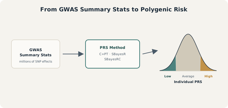
The whole tutorial in one picture: millions of small GWAS effects, combined by a PRS method, collapse into a single number per person – which is only useful once you can place that person in a risk distribution.
GWAS PRS SBayesRC PLINK
0.1 Why Polygenic Risk Scores?
Mendelian diseases (Huntington’s, cystic fibrosis, sickle cell anemia) are driven by mutations in a single gene. Most common diseases aren’t — height, BMI, coronary artery disease, schizophrenia, and depression are each influenced by thousands of variants, each with a tiny individual effect (polygenicity). No single SNP is informative enough to predict risk on its own, which raises the question: how do we combine thousands of tiny genetic effects into a useful predictor? A Polygenic Risk Score (PRS) — also called a Polygenic Score (PGS) — is the answer: a weighted sum of genetic variants across the genome, condensing an individual’s inherited predisposition into a single number.
0.2 What Is a PRS?
\[\text{PRS}_i = \sum_{j=1}^{m} \hat\beta_j\, x_{ij}\]
where \(i\) indexes the individual, \(j\) indexes the SNP, \(m\) is the number of SNPs, \(x_{ij} \in \{0,1,2\}\) is the individual’s risk-allele count at SNP \(j\), and \(\hat\beta_j\) is that SNP’s estimated effect size — usually taken directly from GWAS summary statistics. Positive \(\beta\) increases risk; negative \(\beta\) decreases it.
Worked example. Given effects \(\beta_{rs1}=0.05\), \(\beta_{rs2}=0.02\), \(\beta_{rs3}=-0.03\), and an individual with genotype counts 2, 1, 0:
\[\text{PRS} = (0.05)(2) + (0.02)(1) + (-0.03)(0) = 0.12\]
0.3 Why PRS Works Despite Tiny, Often Non-Causal SNPs
Most SNPs used in a PRS aren’t themselves causal — they still improve prediction because of Linkage Disequilibrium (LD), the tendency of nearby SNPs to be co-inherited. Even without observing the true causal SNP directly, an observed SNP correlated with it still carries predictive information. This is the same principle underlying GWAS itself.
Analogy: a genetic credit score. Just as a bank doesn’t judge creditworthiness from one transaction but aggregates many small signals, a PRS aggregates many small genetic signals into one composite score.
\[\text{Discovery GWAS} \rightarrow \text{Effect Sizes} \rightarrow \text{Target Genotypes} \rightarrow \text{PRS}\]
The discovery dataset produces GWAS effect sizes; the target dataset provides the genotypes (\(x_{ij}\)) of new individuals the score will be applied to. The GWAS effect sizes are simply applied to the target genotypes using the PRS formula above.
0.4 What a PRS Does and Doesn’t Mean
A PRS is not a diagnosis and does not directly measure disease. It represents relative inherited genetic predisposition compared with others in the population — environmental factors still play a major role in whether disease actually develops.
Applications: cardiovascular medicine (identifying individuals with elevated genetic risk for early intervention), and more broadly across common disease research.
Limitations: prediction accuracy is fundamentally capped by the trait’s heritability, GWAS discovery sample size, and how well the discovery population’s ancestry matches the target population (Part 9 covers this in depth).
Key takeaways. A PRS is a weighted sum of genotype counts and GWAS effect sizes across many SNPs. It works even for non-causal SNPs because of LD with true causal variants. A PRS reflects relative genetic predisposition, not a diagnosis, and its accuracy is bounded by heritability and by how well discovery and target populations match.
1 Evaluating Polygenic Risk Scores
A PRS is only useful if it actually predicts the trait — so how well it predicts must be measured rigorously, on held-out data, using metrics that suit the outcome type.
1.1 Quantitative Traits: R² and Incremental R²
For continuous traits (height, BMI, LDL), the standard metric is R², the proportion of phenotypic variance explained. Fit a null model with covariates only, then a full model adding the PRS:
\[\text{Null: Phenotype} \sim \text{Age} + \text{Sex} + \text{PCs}\] \[\text{Full: Phenotype} \sim \text{Age} + \text{Sex} + \text{PCs} + \text{PRS}\]
\[\text{Incremental } R^2 = R^2_{\text{Full}} - R^2_{\text{Null}}\]
This isolates the variance explained specifically by genetics, over and above known covariates.
from sklearn.linear_model import LinearRegression
from sklearn.metrics import r2_score

null_model.fit(X_cov, y)
r2_null = r2_score(y, null_model.predict(X_cov))

full_model.fit(X_full, y)
r2_full = r2_score(y, full_model.predict(X_full))

incremental_r2 = r2_full - r2_null
1.2 Disease Traits: AUC, Pseudo-R², Liability-Scale R²
Binary case/control outcomes need logistic regression and different metrics:
- Pseudo-R² (McFadden, Nagelkerke, Cox-Snell) — analogous to R² but derived from a logistic model; interpretation differs from linear R², but larger is still better.
- AUC (Area Under the ROC Curve) — the probability that a randomly chosen case receives a higher predicted risk than a randomly chosen control.
| AUC | Interpretation |
|---|---|
| 0.50 | Random guessing |
| 0.60 | Weak |
| 0.70 | Moderate |
| 0.80 | Strong |
| 0.90 | Excellent |
from sklearn.metrics import roc_auc_score
auc = roc_auc_score(y_true, prs_scores)
Real-world AUCs vary widely by trait and method: basic clumping-and-thresholding PRS for coronary artery disease or type 2 diabetes often land around 0.57–0.60, while well-optimized, large-biobank PRS have reported AUCs as high as 0.79–0.81 for coronary artery disease. There’s no single “typical” number — it depends heavily on trait architecture, discovery sample size, and how the PRS was built.
- Liability-scale R² — case/control samples are usually enriched for cases relative to the true population prevalence, so raw R² on the observed scale can be misleading. The liability threshold model treats disease as arising once an underlying continuous liability (genetics + environment + noise) crosses a threshold; liability-scale R² estimates the proportion of that underlying liability explained by the PRS. This metric is especially common in psychiatric genetics.
1.3 Risk Stratification and Odds Ratios
Individuals are commonly split into PRS groups — deciles are typical — and disease prevalence compared across groups. Example: bottom decile odds ratio = 1.0 (reference), top decile odds ratio = 3.5, meaning individuals in the top PRS decile have 3.5× the disease odds of those in the bottom decile. A useful PRS shows monotonically increasing risk from lowest to highest group.
1.4 Avoiding Overfitting: Discovery, Tuning, and Target Sets
A major pitfall: building a PRS, testing many parameter choices, picking the best-performing one, and evaluating on the same individuals used for tuning — this inflates the apparent accuracy, because the model has effectively already “seen” the answer. The standard fix is three independent datasets:
| Dataset | Role |
|---|---|
| Discovery | Runs the GWAS, produces SNP effect estimates |
| Tuning | Optimizes parameters (p-value thresholds, clumping settings, hyperparameters) |
| Target | Used once, to report final unbiased prediction performance |
If individuals overlap between discovery and target sets, prediction accuracy is artificially inflated. These three samples must remain independent — this is the gold standard for reporting PRS performance.
Key takeaways. Quantitative traits are evaluated with incremental R²; disease traits with AUC, pseudo-R², liability-scale R², and odds ratios. Risk stratification (typically by decile) gives an intuitive picture of prediction performance. Overfitting from re-using tuning data is one of the most common and serious mistakes in PRS evaluation — discovery, tuning, and target datasets must stay independent.
2 Clumping and P-Value Thresholding (C+PT)
Given GWAS summary statistics, how do we decide which SNPs actually go into a PRS? Naively including every SNP creates problems: many SNPs are highly correlated via LD, many have noisy or negligible effect estimates, and millions of SNPs together introduce substantial statistical noise. Clumping and P-value Thresholding (C+PT) was one of the earliest and most influential answers to this, and despite newer Bayesian methods, it remains a widely used baseline.
2.1 Why Not Just Use Every SNP?
A GWAS hit on chromosome 6 might show 5 SNPs all with p-values around \(10^{-10}\)–\(10^{-12}\) — not 5 independent discoveries, but the same underlying signal viewed through SNPs inherited together via LD. Including all of them in a PRS effectively double- (or quintuple-) counts the same genetic information, producing redundant information, inflated variance, overfitting, and reduced prediction accuracy.
2.2 The Two-Step Procedure
\[\text{GWAS Summary Statistics} \rightarrow \text{Clumping} \rightarrow \text{P-value Thresholding} \rightarrow \text{Final SNP Set} \rightarrow \text{Polygenic Score}\]
Step 1 — Clumping removes redundant SNPs, keeping the most significant SNP in each LD region and discarding its correlated neighbors:
- Sort SNPs by p-value (most significant first).
- Select the most significant remaining SNP.
- Remove all SNPs within a specified window (e.g. 250 kb) whose LD with it exceeds a threshold (e.g. \(r^2 > 0.1\)).
- Move to the next remaining SNP and repeat until all SNPs are processed.
| \(r^2\) threshold | Interpretation |
|---|---|
| 0.1 | Strict — removes more SNPs |
| 0.2 | Moderate |
| 0.5 | Relaxed |
Step 2 — P-value thresholding. After clumping, still-many SNPs must be filtered by significance. Researchers typically test several thresholds — \(5\times10^{-8}\), \(10^{-6}\), \(10^{-4}\), \(10^{-2}\), 0.05, 0.1, 0.5, 1.0 — and pick whichever gives the best held-out prediction. Restricting to genome-wide-significant SNPs alone (\(P < 5\times10^{-8}\)) is tempting but usually suboptimal for highly polygenic traits: many true causal variants never individually reach that threshold, so overly strict cutoffs discard real signal.
The tuning process. Compare incremental \(R^2\) across thresholds on a tuning set:
| Threshold | Incremental R² |
|---|---|
| 5e-8 | 0.03 |
| 1e-6 | 0.05 |
| 1e-4 | 0.08 |
| 0.01 | 0.11 |
| 0.05 | 0.09 |
Here 0.01 wins. This produces the classic hump-shaped curve: too few SNPs misses real signal (low accuracy), a moderate number captures the optimal balance (peak accuracy), and too many SNPs lets noise dominate (accuracy falls again).
2.3 Scoring and Practical Use
The final score uses the same formula as before, restricted to the selected SNP set:
\[\text{PRS}_i = \sum_{j=1}^{m} \hat\beta_j\, x_{ij}\]
plink \
  --bfile target_data \
  --score selected_snps.txt 1 2 3 \
  --out prs_scores
(Column 1 = SNP ID, column 2 = effect allele, column 3 = effect size — PLINK multiplies genotype counts by effects and sums.)
2.4 Strengths and Limitations
Strengths: simple, computationally cheap, works directly from summary statistics, easy to reproduce — hence its continued use as the standard baseline. Limitations: discards potentially useful SNPs during clumping, handles LD only indirectly (via pruning, not explicit modeling), treats each SNP’s effect independently rather than jointly, and requires threshold tuning (adding complexity and overfitting risk).
These limitations motivated whole-genome regression and Bayesian methods — BLUP, SBLUP, LDpred, BayesR, BayesC, SBayesR, SBayesRC — which use all SNPs, model LD directly, and apply shrinkage. C+PT nonetheless remains the essential conceptual starting point for understanding them.
Key takeaways. C+PT selects SNPs in two steps: clumping removes LD-redundant SNPs, and p-value thresholding filters by significance, typically tuned across several candidate cutoffs. Prediction accuracy follows a hump-shaped curve against threshold stringency. C+PT is simple and widely used, but discards information and ignores joint LD structure — limitations that motivated modern Bayesian PRS methods.
3 Best Linear Unbiased Prediction (BLUP)
C+PT discards many SNPs, ignores joint LD structure, treats SNPs independently, and requires threshold tuning. BLUP represents a conceptual shift: use every SNP simultaneously rather than selecting a subset. Understanding BLUP matters because modern Bayesian methods (BayesR, SBayesR) are direct extensions of it.
3.1 The Infinitesimal Model
BLUP rests on one of the oldest ideas in quantitative genetics — the infinitesimal model: every SNP contributes to the trait, each with a very small effect, drawn from a shared normal distribution \(\beta_j \sim N(0, \sigma_\beta^2)\). Most SNP effects cluster near zero, symmetric around it, with very large effects rare. This is a surprisingly good approximation for many highly polygenic traits (height, BMI, schizophrenia — GWAS repeatedly show thousands of associated variants each).
“Best Linear Unbiased Prediction” breaks down as: Best = smallest prediction error variance among linear unbiased estimators; Linear = prediction is a linear combination of SNP effects (\(\hat y = X\hat\beta\)); Unbiased = predictions aren’t systematically too high or too low.
3.2 The Mixed Model Framework
\[y = Xb + Zu + e\]
\(Xb\) are fixed effects (known covariates like age, sex, principal components, batch); \(Zu\) is the genetic component, treated as a random effect: \(u \sim N(0, G\sigma_g^2)\), where \(G\) is the Genetic Relationship Matrix (GRM) — pairwise genetic similarity between individuals — and \(\sigma_g^2\) is genetic variance. Rather than estimating each SNP’s effect independently, BLUP models their collective contribution via this relationship structure: more genetically similar individuals are expected to be more phenotypically similar.
3.3 Shrinkage
BLUP doesn’t trust raw GWAS estimates fully — it pulls them toward zero, more aggressively for small/noisy estimates than large ones. Example: GWAS effects of 0.40, 0.05, 0.01 might become BLUP effects of 0.25, 0.03, 0.005. Because small-sample GWAS estimates can be inflated by chance, shrinkage separates “mostly signal” from “signal + noise,” reducing overfitting and improving out-of-sample prediction.
PRS calculation is otherwise unchanged — \(\text{PRS}_i = \sum_j \hat\beta_j x_{ij}\) — the difference from C+PT is simply that every SNP contributes, not a selected subset.
3.4 Advantages and Limitations
Advantages: uses all SNPs (no discarding), no arbitrary p-value thresholds to tune, handles polygenicity naturally, and shrinkage reduces overfitting.
Limitations: assumes every SNP has a non-zero effect (unrealistic — many SNPs likely have none), assumes a single normal distribution for all effects (real traits likely have null, small-, medium-, and large-effect SNP classes that a single distribution can’t represent), and struggles to incorporate sparse architectures or functional annotations.
| Feature | C+PT | BLUP |
|---|---|---|
| Uses all SNPs | No | Yes |
| Requires tuning | Yes | No |
| Models LD directly | Partially | Better |
| Shrinkage | No | Yes |
| Computational complexity | Low | Moderate |
BLUP’s single-distribution assumption motivated researchers to ask: what if many SNPs truly have zero effect, effect sizes come from multiple distributions, or biological annotations could be incorporated? Answering these questions led to Bayesian methods (BayesA, BayesB, BayesC, BayesR, SBayesR, SBayesRC) — direct generalizations of the BLUP framework that relax its restrictive assumptions.
Key takeaways. BLUP is a whole-genome regression method using all SNPs simultaneously, under the infinitesimal-model assumption that effects are normally distributed. It relies on a Genetic Relationship Matrix and applies shrinkage to reduce overfitting, eliminating the need for clumping or p-value thresholds. Its core limitation — one shared normal distribution for every SNP effect — motivated the Bayesian methods that followed.
4 Bayesian Methods and MCMC
BLUP’s key limitation is assuming every SNP’s effect is drawn from one shared normal distribution — unrealistic, since many SNPs likely have zero effect while a few have outsized ones. Bayesian methods relax this by treating SNP effects as random variables with more flexible priors — the foundation for BayesA, BayesB, BayesC, BayesR, and their modern summary-statistics descendants SBayesR and SBayesRC.
4.1 The Bayesian Philosophy
Classical (frequentist) statistics treats a parameter like \(\beta\) as a fixed but unknown true value. Bayesian statistics instead asks for its full probability distribution, combining:
- Prior beliefs — what we assume before seeing data, e.g. \(\beta_j \sim N(0, \sigma^2)\), encoding “most effects are small, positive and negative are equally likely, large effects are rare.”
- The likelihood — how probable the observed data is under a given parameter value.
via Bayes’ theorem: \(\text{Posterior} \propto \text{Prior} \times \text{Likelihood}\). If the prior expects \(\beta \approx 0\) but the GWAS data strongly suggests \(\beta \approx 0.3\), the posterior lands somewhere in between (e.g. \(\beta \approx 0.2\)) — naturally shrinking noisy GWAS estimates toward more plausible values, which often improves prediction.
4.2 BayesC and the Spike-and-Slab Prior
BayesC was the first influential model of this kind: some SNPs have exactly zero effect (\(\beta_j = 0\), probability \(\pi\)), others are drawn from a normal distribution (\(\beta_j \sim N(0,\sigma_\beta^2)\), probability \(1-\pi\)). This is a spike-and-slab prior — a “spike” at zero for null SNPs, a “slab” (broader distribution) for real effects. Rather than forcing every SNP to contribute, BayesC lets the data determine which SNPs matter, reducing noise and improving shrinkage — especially when the true genetic architecture is sparse (e.g. 100 causal variants among 1,000,000 measured SNPs, which BLUP handles poorly).
4.3 Why MCMC Is Needed
Bayesian posteriors for a million SNPs at once have no closed-form solution — the parameter space is far too high-dimensional to compute directly. Markov Chain Monte Carlo (MCMC) solves this by sampling from the posterior instead of solving it analytically. It combines two ideas: a Markov chain (each new state depends only on the current state, not the full history) and Monte Carlo sampling (random draws used to approximate otherwise intractable quantities, in the spirit of estimating \(\pi\) by randomly throwing darts at a circle inscribed in a square). Over many iterations, MCMC spends more time in high-posterior-probability regions and less in low-probability ones, and the accumulated samples reconstruct the posterior distribution.
Gibbs sampling is the standard MCMC algorithm here: rather than updating SNP effects (\(\beta\)), genetic variance (\(\sigma_\beta^2\)), residual variance (\(\sigma_e^2\)), and the inclusion probability (\(\pi\)) all simultaneously, it updates them one at a time, cycling through thousands of iterations:
Update β → Update σ²β → Update σ²e → Update π → repeatBurn-in. Early samples reflect arbitrary starting values rather than the true posterior, so they’re discarded — e.g. of 50,000 total iterations, the first 10,000 might be burn-in, leaving 40,000 retained samples for inference.
Convergence diagnostics. A trace plot (parameter value vs. iteration) that fluctuates stably around a constant mean suggests convergence; a plot with a clear upward/downward trend suggests the chain hasn’t stabilized yet.
Extracting estimates. After convergence, the posterior mean \(\bar\beta = \frac{1}{N}\sum_i \beta^{(i)}\) becomes the final SNP effect estimate, and posterior variance quantifies uncertainty (large variance = low confidence). A SNP’s Posterior Inclusion Probability (PIP) is simply the fraction of retained iterations in which it was included — e.g. included in 45,000 of 50,000 samples gives PIP = 0.90.
| PIP | Interpretation |
|---|---|
| 0.01 | Almost certainly irrelevant |
| 0.10 | Weak evidence |
| 0.50 | Moderate evidence |
| 0.90 | Strong evidence |
| 0.99 | Very strong evidence |
4.4 Strengths, Weaknesses, and the Path Forward
MCMC provides full posterior distributions, honest uncertainty estimates, and PIPs — real advantages over point-estimate methods. But it’s also computationally expensive (1 million SNPs × 50,000 iterations can take hours to days and substantial memory), can converge slowly, and can be hard to diagnose. This computational burden directly motivated SBayesR and SBayesRC, which achieve similar Bayesian flexibility using summary statistics and efficient sparse-matrix methods instead of raw individual-level MCMC over the full genotype matrix.
Key takeaways. Bayesian methods treat SNP effects as random variables with flexible priors rather than a single shared distribution. BayesC’s spike-and-slab prior lets some SNPs have exactly zero effect. Because the resulting posteriors have no closed-form solution, MCMC (typically Gibbs sampling) approximates them via iterative random sampling, discarding early “burn-in” draws and using posterior means and inclusion probabilities as final estimates. MCMC’s computational cost motivated the summary-statistics-based methods that followed.
5 SBayesR: Bayesian Prediction from Summary Statistics
MCMC over individual-level genotypes is powerful but computationally expensive at biobank scale. SBayesR (summary-data-based BayesR) reformulates the BayesR model to run on GWAS summary statistics plus an LD reference panel, instead of raw genotypes — making Bayesian polygenic prediction tractable at scale. It’s now one of the most widely used methods for building PRS from GWAS summary data, and the foundation for SBayesRC.
5.1 Why SBayesR Was Developed
Each earlier method had a specific gap: C+PT discards SNPs and ignores joint LD; BLUP forces every SNP into a single effect-size distribution; individual-level BayesC models sparsity well but needs raw genotype data and is computationally expensive at scale. Researchers wanted Bayesian flexibility, summary-statistics compatibility, and scalability together — SBayesR was the answer, implemented in the GCTB software.
5.2 The Mixture Prior
BLUP assumes one shared distribution, \(\beta_j \sim N(0,\sigma_\beta^2)\), for every SNP. BayesR (and SBayesR) instead uses a mixture of normal distributions with a point mass at zero:
\[\beta_j \sim \sum_{k=1}^{K} \pi_k\, N(0, \gamma_k \sigma_\beta^2)\]
where \(\pi_k\) is the proportion of SNPs in class \(k\) and \(\gamma_k\) scales that class’s variance. The standard BayesR/SBayesR configuration uses four components — \(\gamma = (0,\ 0.01,\ 0.1,\ 1)\) — representing zero effect, small effect, medium effect, and large effect classes respectively (component 1 is a literal point mass at zero; components 2–4 scale \(\sigma_\beta^2\) by 0.01×, 0.1×, and 1× respectively). A typical starting mixture might set \(\pi = (0.95,\ 0.02,\ 0.02,\ 0.01)\) — most SNPs assigned near-zero effect, a small number carrying most of the real signal — and SBayesR estimates the actual proportions from the data during MCMC, which itself provides insight into the trait’s genetic architecture.
5.3 Recovering Joint Effects from Marginal GWAS Statistics
GWAS summary statistics report marginal effects — each SNP tested one at a time, ignoring correlation with its neighbors. The relationship to the true joint effects is approximately \(b = R\beta + \epsilon\), where \(b\) is the vector of observed GWAS effects, \(R\) is the LD matrix, and \(\beta\) is the joint effect vector SBayesR aims to recover. If rs1, rs2, rs3 are strongly correlated, a naive analysis might spread signal across all three; modeling them jointly through \(R\) lets SBayesR assign most of the signal to one and shrink the others toward zero — improving both interpretability and prediction.
5.4 Making This Computationally Tractable
A full LD matrix for 1 million SNPs has \(10^{12}\) entries — far too large to handle directly. Because most SNPs are only correlated with nearby variants, the vast majority of LD matrix entries are effectively zero, so SBayesR stores a sparse representation (reduced memory, faster computation), and can further use an eigen-decomposition \(R = U\Lambda U^T\) to reduce the computational burden during MCMC sampling. These optimizations are what make biobank-scale SBayesR analyses feasible at all.
5.5 Running SBayesR
gctb \
  --sbayes R \
  --ldm ukbEURu_hm3_sparse \
  --gwas-summary trait.ma \
  --out trait_sbayesr
Internally, GCTB reads the summary statistics, loads the LD matrix, runs MCMC (updating SNP effects, mixture-component membership, genetic variance, and residual variance each iteration), and outputs posterior mean SNP effects to trait_sbayesr.snpRes and MCMC/parameter diagnostics to trait_sbayesr.parRes. These posterior effects are typically less noisy than raw GWAS effects, and are combined with target genotypes using PLINK’s --score, exactly as in earlier methods.
5.6 Strengths and Limitations
Strengths: uses all SNPs, models LD directly (joint rather than marginal effects), a flexible mixture prior that better matches real genetic architecture, works from summary statistics alone, and scales to biobank-sized analyses.
Limitations: treats every SNP as equally likely to be causal a priori — no biological information about coding regions, regulatory elements, or conservation is used; results depend on how well the LD reference panel matches the GWAS population; and it remains more computationally demanding than C+PT.
| Feature | C+PT | BLUP | SBayesR |
|---|---|---|---|
| Uses all SNPs | No | Yes | Yes |
| Models LD | Partial | Better | Yes (jointly) |
| Summary statistics only | Yes | No | Yes |
| Mixture prior | No | No | Yes |
| Sparse architecture | No | No | Yes |
That first limitation — ignoring biology — is exactly what SBayesRC addresses next.
Key takeaways. SBayesR extends BayesR to work from GWAS summary statistics and an LD reference panel, using a four-component mixture prior (a zero-effect spike plus three non-zero variance classes) instead of BLUP’s single normal distribution. Sparse LD matrices and eigen-decomposition make this tractable at biobank scale. It doesn’t yet use any biological/functional information — the motivation for SBayesRC.
6 SBayesRC: Adding Functional Annotations
SBayesR treats every SNP as equally likely to be causal before seeing the data — but decades of molecular biology say that’s not realistic. A SNP sitting in a protein-coding exon and a SNP sitting in an intergenic region shouldn’t necessarily get the same prior probability of being causal, even with identical GWAS p-values. SBayesRC extends SBayesR by letting functional annotations inform those priors.
6.1 Functional Annotations and Heritability Enrichment
Functional annotations describe biological properties of genomic regions — coding sequence, promoters, enhancers, evolutionarily conserved regions, open chromatin (DNase hypersensitivity sites), histone marks, and more. Each SNP can be tagged with one or more of these categories, forming an annotation matrix (SNP × annotation, 0/1 entries).
The key concept is heritability enrichment: some annotation categories explain disproportionately more heritability than their share of the genome would suggest. Illustratively:
| Annotation | SNP Fraction | Heritability Fraction | Enrichment |
|---|---|---|---|
| Coding | 2% | 10% | 5× |
| Conserved | 5% | 20% | 4× |
| Intergenic | 50% | 20% | 0.4× |
\[\text{Enrichment} = \frac{\text{Heritability Proportion}}{\text{SNP Proportion}}\]
An enrichment of 5 means that annotation category contributes five times more heritability than its size alone would predict — flagging it as more likely to harbor causal variants, and letting SBayesRC assign it a higher prior probability of non-zero effect during inference.
6.2 The Model Change
In SBayesR, the mixture-component probabilities \(\pi_k\) are the same for every SNP. In SBayesRC, \(\pi_k\) becomes a function of each SNP’s annotations — so two SNPs with identical GWAS evidence can receive different prior probabilities of being causal, depending on their biological context. This lets SBayesRC combine statistical evidence and biological plausibility, rather than statistical evidence alone.
6.3 Running SBayesRC
gctb \
  --sbayes RC \
  --ldm ukbEURu_hm3_sparse \
  --annot annotations.txt \
  --gwas-summary trait.ma \
  --out trait_sbayesrc
The only new input compared with SBayesR is the annotation file. Large-scale implementations commonly draw on baselineLD-style annotation sets spanning coding regions, conservation, regulatory elements, histone modifications, and gene expression — often dozens to hundreds of categories. Typical outputs add trait_sbayesrc.enrich, summarizing annotation-specific heritability enrichment, alongside the usual .snpRes and .parRes files.
6.4 Advantages and Limitations
Because it draws on both statistical and biological evidence, SBayesRC often modestly but consistently outperforms SBayesR across traits. That said, it inherits new failure modes: annotation quality directly affects performance (poor annotations can hurt more than help); it estimates more parameters, adding computational cost; annotations may not transfer cleanly across ancestries; and even the best current annotation sets capture only a fraction of real regulatory biology.
| Feature | SBayesR | SBayesRC |
|---|---|---|
| Summary statistics | Yes | Yes |
| LD modeling | Yes | Yes |
| Mixture priors | Yes | Yes |
| Functional annotations | No | Yes |
| Heritability enrichment | No | Yes |
Key takeaways. SBayesRC extends SBayesR by letting functional annotations modify each SNP’s prior probability of being causal, using heritability enrichment to identify biologically important genomic regions. Combining statistical and biological evidence often modestly improves prediction accuracy over SBayesR alone — though results still depend on annotation quality and completeness, and may not generalize equally across ancestries.
7 Practical PRS Analysis: PRSice, GCTB, PLINK
A complete PRS pipeline, connecting the theory above to actual tools:
\[\text{Discovery GWAS} \rightarrow \text{Summary Stats QC} \rightarrow \text{PRS Method (C+PT / SBayesR / SBayesRC)} \rightarrow \text{Posterior SNP Effects} \rightarrow \text{PLINK Scoring} \rightarrow \text{Prediction Evaluation}\]
7.1 Required Datasets and Files
Three datasets, as in Part 2: discovery (produces GWAS summary statistics), target (genotypes, phenotypes, covariates for evaluation), and an LD reference for methods that need it (SBayesR, SBayesRC, LDpred) — commonly UK Biobank, 1000 Genomes, or HapMap3.
A typical project layout:
GWAS/         trait.ma
Target/       target.bed, target.bim, target.fam
Covariates/   covariates.txt
Phenotypes/   phenotype.txt
LD/           ukb_ldm/
7.2 Step 1 — QC Summary Statistics and Target Genotypes
Check for missing SNP IDs, duplicate variants, strand ambiguity, allele mismatches, and incorrect sample sizes in the summary statistics — poor-quality summary stats reliably wreck downstream prediction.
plink \
  --bfile target \
  --geno 0.02 \
  --mind 0.02 \
  --maf 0.01 \
  --make-bed \
  --out target_QC
7.3 Step 2 — C+PT via PRSice
PRSice implements clumping, thresholding, PRS construction, and evaluation in one tool:
Rscript PRSice.R \
  --prsice PRSice_linux \
  --base trait.ma \
  --target target_QC \
  --pheno phenotype.txt \
  --cov covariates.txt \
  --stat BETA \
  --beta \
  --out PRS_output
--base is the GWAS summary file, --target the target genotypes, --pheno/--cov the phenotype and covariates for evaluation. Outputs include PRS_output.best (best p-value threshold), PRS_output.summary (incremental R², SNP counts), and PRS_output.all_score (scores at every threshold tested).
7.4 Step 3 — SBayesR and SBayesRC via GCTB
GCTB needs an LD reference matrix in addition to summary statistics — pre-computed sparse LD matrices derived from UK Biobank reference panels (e.g. ukbEURu_hm3_sparse) are commonly used:
gctb \
  --sbayes R \
  --ldm ukbEURu_hm3_sparse \
  --gwas-summary trait.ma \
  --out trait_sbayesr
For SBayesRC, add an annotation file and switch --sbayes R to --sbayes RC:
gctb \
  --sbayes RC \
  --ldm ukbEURu_hm3_sparse \
  --annot annotations.txt \
  --gwas-summary trait.ma \
  --out trait_sbayesrc
Both produce a .snpRes file with posterior SNP effects, generally less noisy than raw GWAS betas.
7.5 Step 4 — Scoring and Evaluation
plink \
  --bfile target_QC \
  --score score.txt 1 2 3 \
  --out target_PRS
producing per-individual scores (FID IID SCORE1_SUM). Evaluate exactly as in Part 2 — compare a full model (Phenotype ~ Sex + Age + PCs + PRS) against a null model (Phenotype ~ Sex + Age + PCs) and take the incremental \(R^2\):
null_model.fit(X_cov, y);  r2_null = r2_score(y, null_model.predict(X_cov))
full_model.fit(X_full, y); r2_full = r2_score(y, full_model.predict(X_full))
incremental_r2 = r2_full - r2_null
Then stratify by risk group (e.g. bottom 10% / middle 80% / top 10%) and compare disease prevalence across them.
Illustrative method comparison (values are trait-dependent, not universal constants):
| Method | Incremental R² |
|---|---|
| C+PT | 0.08 |
| BLUP | 0.10 |
| SBayesR | 0.13 |
| SBayesRC | 0.14 |
SBayesRC often — not always — achieves the highest accuracy among these; the actual ranking depends on the trait, sample size, and annotation quality available.
7.6 Common Problems and Best Practices
Common problems: allele mismatches between summary statistics and target genotypes (the single most frequent source of errors — always harmonize alleles first); an LD reference whose ancestry doesn’t match the GWAS population (degrades accuracy); sample overlap between discovery and target sets (inflates apparent performance); and poor-quality input summary statistics (garbage in, garbage out).
Best practices: thorough QC at every step, ancestry-matched LD references, strict independence between discovery/tuning/target samples, evaluation only on held-out data, and comparing multiple methods rather than trusting one blindly.
Key takeaways. PRSice runs C+PT end-to-end; GCTB runs SBayesR (
--sbayes R) and SBayesRC (--sbayes RC, plus--annot); PLINK’s--scoreconverts posterior SNP effects into individual-level PRS. Allele mismatches and LD reference mismatch are the most common practical failure points — careful QC and ancestry matching matter as much as method choice.
8 Interpreting PRS: What Do They Really Mean?
A high PRS does not mean “you will get the disease,” and a low PRS does not mean “you’re protected.” Both are common misreadings. A PRS is a statistical predictor, not a diagnosis — understanding its actual meaning matters for responsible use in research, medicine, and public communication.
8.1 Relative Position, Not Absolute Fate
A PRS represents an individual’s genetic predisposition relative to others in the same population — the operative word is relative. A height-PRS analogy: knowing Person C’s PRS is +2.4 and Person A’s is −2.1 doesn’t tell you their exact heights, but does suggest Person C is likely taller than Person A. The same logic carries over to disease risk.
8.2 Relative Risk vs. Absolute Risk
These two are frequently conflated. If average disease risk is 10% and the top PRS decile has “3× higher risk” (a relative risk statement), the absolute risk for that group becomes roughly 30% — meaningfully elevated, but nowhere near certainty. Even high-risk individuals usually don’t develop the disease. This distinction is essential when communicating PRS results to anyone outside a statistics-fluent audience.
8.3 Percentiles Make Raw Scores Interpretable
A raw score like “PRS = 1.42” means almost nothing by itself — interpretation improves enormously once it’s expressed as a percentile within a reference population (e.g. 99th percentile = higher than 99% of people). Most PRS distributions are approximately normal, with most individuals clustering near the middle and extreme scores becoming rarer toward the tails.
Illustrative risk stratification example (coronary artery disease):
| Group | Disease Rate |
|---|---|
| Bottom 10% | 3% |
| Average | 7% |
| Top 10% | 18% |
Higher PRS tracks with higher disease frequency, but the majority of even the top-decile group still doesn’t develop the disease. Odds ratios (e.g. top decile 3.5× the odds of bottom decile) summarize this pattern compactly, but odds and probability aren’t the same thing and shouldn’t be conflated.
8.4 PRS Is Not Destiny
Phenotype = Genetics + Environment + Random effects, roughly speaking — even highly heritable diseases have substantial non-genetic contributors. For type 2 diabetes, diet, physical activity, obesity, smoking, and sleep all matter alongside genetic risk: a high-PRS individual may never develop disease, and a low-PRS individual isn’t guaranteed protection.
Heritability sets a hard ceiling. If a trait’s heritability is \(h^2 = 0.40\), only 40% of phenotypic variation is genetic in origin — even a theoretically perfect PRS cannot explain the other 60%, because that variance simply isn’t genetic. A high PRS suggests increased inherited susceptibility and elevated relative risk; it does not imply certainty of disease, an immediate clinical diagnosis, or the presence of symptoms.
8.5 Population Portability
A PRS trained on a European-ancestry GWAS and applied to an African-ancestry population typically loses substantial predictive accuracy — driven by differing allele frequencies, differing LD patterns (so tag SNPs correlated with a causal variant in one population may be poorly correlated with it in another), and differing environmental exposures. This portability problem is one of the major open challenges in the field (Part 10 covers it further).
8.6 Clinical and Ethical Considerations
Potential clinical uses include early screening, targeting preventive interventions, and risk communication as part of personalized medicine — but clinical implementation is still an active area of research, not settled practice. PRS should be one input among many (family history, lifestyle, environmental exposures, medical records, biomarkers), not a standalone basis for major decisions. Open ethical questions include data privacy, potential for discrimination (e.g. insurance, employment), how to communicate risk responsibly, and equitable distribution of benefit across ancestries currently underrepresented in GWAS.
8.7 Common Misinterpretations, Corrected
| Misinterpretation | Reality |
|---|---|
| High PRS = disease | False — it’s elevated relative risk, not certainty |
| Low PRS = protected | False — non-genetic factors still matter |
| Genetics = destiny | False — environment and chance both contribute substantially |
| PRS works equally in every population | False — accuracy varies by ancestry match to the discovery GWAS |
Key takeaways. A PRS measures relative genetic predisposition, not a diagnosis. Relative risk and absolute risk are different quantities and shouldn’t be conflated; percentiles are usually more interpretable than raw scores. Prediction accuracy is capped by heritability and degrades when applied across ancestries different from the discovery GWAS. Responsible use treats PRS as one input among several, not a standalone predictor of fate.
9 The Future of PRS: Multi-Ancestry, Functional Genomics, Precision Medicine
Despite real progress — from simple weighted sums to SBayesRC’s Bayesian, LD-aware, annotation-informed models — today’s PRS methods remain far from perfect. Major open challenges: limited cross-ancestry portability, missing heritability, gene-environment interactions, rare variants, and clinical implementation.
Prediction accuracy today varies substantially by trait: it’s generally strongest for traits like height, and more modest for BMI, coronary artery disease, type 2 diabetes, schizophrenia, and especially depression — reflecting real differences in genetic architecture, GWAS sample size, and environmental contribution across traits, not just tool limitations.
9.1 The Multi-Ancestry Problem
Most large GWAS to date have been conducted in European-ancestry cohorts, so PRS trained on them predict well within European-ancestry populations but substantially worse when applied to other ancestries. Three main drivers: differing allele frequencies (a SNP common in one population may be rare in another, changing its statistical power to contribute to prediction); differing LD patterns (a tag SNP correlated with a causal variant in one population may be weakly correlated with it in another, breaking the LD-based logic PRS relies on); and differing environmental exposures (diet, healthcare access, socioeconomic conditions), meaning even identical genetics can translate to different outcomes.
Multi-ancestry PRS methods, combining GWAS data across ancestral groups and modeling both shared and population-specific genetic effects, are an active area of development aimed at improving generalization — though this remains one of the field’s largest unsolved problems, and the underrepresentation of non-European ancestries in existing GWAS is a structural, not just methodological, limitation.
9.2 Larger Samples, Rarer Variants
Prediction accuracy scales with discovery GWAS sample size. Major biobanks now include roughly: UK Biobank (~500,000 participants), FinnGen (~500,000), the Million Veteran Program (over 1,000,000), and All of Us (targeting over 1,000,000) — with future resources likely to grow substantially larger still.
Most current PRS focus on common variants; rare variants may carry larger individual biological effects but are harder for standard GWAS to detect reliably, since statistical power drops sharply as allele frequency falls. Integrating common, rare, and structural variation into a single predictive framework is an active research direction.
9.3 Functional Genomics and Multi-Omics
Beyond the coding/regulatory annotations SBayesRC already uses, future models may incorporate gene expression (eQTLs), chromatin accessibility, single-cell-resolved cell-type-specific effects, and epigenetic marks (DNA methylation, histone modifications) — moving toward genuinely multi-omics prediction. Related approaches like TWAS (transcriptome-wide association studies), PrediXcan, and FUSION predict disease via genetically-predicted gene expression as an intermediate step (SNPs → predicted expression → disease), rather than jumping directly from SNPs to phenotype — potentially yielding more biologically interpretable predictions.
Gene-environment interaction (G×E). Standard PRS models assume genetic and environmental contributions are additive/independent, but reality is often more complex — a genetic predisposition to obesity, for instance, may be amplified by a high-calorie diet and sedentary lifestyle, or dampened by exercise and healthy nutrition. Modeling these interactions explicitly, rather than assuming independence, is an active area of methods development.
9.4 Machine Learning, and What Actually Moves the Needle
Neural networks, graph neural networks, transformer architectures, and other deep-learning approaches are being explored for genomic prediction, offering potential to capture nonlinear effects and integrate heterogeneous data types. So far, though, evidence suggests that for most current PRS applications, better data tends to matter more than more complex models — larger, more diverse, better-QC’d GWAS typically move prediction accuracy further than swapping in a more sophisticated architecture on the same underlying data.
9.5 Clinical Translation
Potential applications span cardiovascular disease (earlier intervention for high-risk individuals), cancer screening (risk-stratified programs), psychiatry (earlier identification of vulnerable individuals), and preventive medicine generally. Real obstacles to clinical adoption remain: calibration (predicted risks must actually match observed outcomes), equity (prediction must work reasonably across diverse populations, not just those well-represented in discovery GWAS), interpretability (clinicians need understandable, actionable outputs), and ethics (privacy and fairness). These are as important to solve as any statistical improvement.
The long-term vision — often called precision medicine — combines individual genome, environment, and medical history into personalized healthcare; PRS is likely to become one input among several in that broader picture, not a stand-alone diagnostic tool.
9.6 How the Field Got Here
| Era | Approach |
|---|---|
| Early | Candidate gene studies |
| GWAS era | Single-SNP association analysis |
| PRS era | C+PT |
| Whole-genome era | BLUP |
| Bayesian era | BayesR |
| Summary-statistics era | SBayesR |
| Functional genomics era | SBayesRC |
Each generation incorporated more information and more realistic assumptions about genetic architecture than the last.
Final key takeaways. PRS is now central to statistical genetics, and accuracy keeps improving as datasets grow — but multi-ancestry portability, missing heritability, gene-environment interactions, and rare variants remain substantial open problems. Deep learning may help at the margins, but data quality and quantity currently matter more than model sophistication. Clinical implementation requires careful validation on calibration, equity, and interpretability, not just prediction accuracy. Precision medicine — integrating genetics, environment, and clinical data — is a long-term goal the field is still working toward, not a present reality.