Structural Equation Modeling: A Practical Tutorial with R

What SEM is, why it matters, and how to fit a model using lavaan

Statistics

Structural Equation Modeling

Latent Variables

Lavaan

Data Science

Author

Nivedita Bhadra

Published

May 28, 2026

1 What is Structural Equation Modeling?

Structural Equation Modeling, usually called SEM, is a statistical framework used to study relationships among multiple variables at the same time.

In ordinary regression, we usually ask a question like:

Does X predict Y? — for example, does stress predict depression score?

SEM lets us ask a broader, more realistic question:

How do several observed and unobserved variables relate to each other simultaneously? Does socioeconomic status influence stress, and does stress then influence depression? Are stress and depression measured through several questionnaire items rather than one direct variable? Is the effect of socioeconomic status on depression partly mediated through stress?

SEM is useful because many scientific concepts are not directly observed. Variables such as intelligence, resilience, depression, socioeconomic status, anxiety, wellbeing, cognitive ability, and biological vulnerability are often latent constructs — we observe them indirectly, through questionnaire items, test scores, biomarkers, or behavioral measures.

SEM combines two ideas:

Measurement model — describes how observed variables measure latent variables.
Structural model — describes how latent or observed variables relate to each other.

A simple way to remember SEM:

SEM = factor analysis + regression/path analysis

The lavaan package is one of the most widely used open-source R packages for SEM. It supports confirmatory factor analysis, SEM, latent growth models, and related latent variable models (Rosseel, 2012, Journal of Statistical Software).

2 Why is SEM important?

SEM matters because many real-world research questions aren’t simple one-variable-to-one-variable problems. In psychology, psychiatry, education, epidemiology, sociology, genetics, public health, and economics, researchers routinely work with complex systems, and SEM helps model them in a structured way.

Suppose we’re studying psychological resilience. We might believe that family support improves resilience, resilience reduces depression, socioeconomic stress reduces resilience, depression is measured by several symptoms, and resilience is measured by several questionnaire items. A basic regression model can only test one piece of this system at a time — SEM lets us test the full hypothesized structure at once.

SEM is especially useful when we want to model latent variables, account for measurement error, test mediation, test direct and indirect effects, combine multiple regression equations, test whether a theoretical model fits the data, or compare competing theoretical models. This is why SEM is common in fields where theoretical structure matters as much as prediction.

3 Observed Variables and Latent Variables

In SEM, variables are usually divided into two types.

3.1 Observed Variables

Observed variables are directly measured in the dataset — age, sex, income, PHQ-9 item scores, test scores, biomarker values, and questionnaire responses are all examples. In path diagrams, observed variables are usually shown as rectangles.

3.2 Latent Variables

Latent variables are not directly observed — they’re inferred from multiple observed indicators. Depression, anxiety, resilience, cognitive ability, socioeconomic status, inflammation, and wellbeing are common examples. In path diagrams, latent variables are usually shown as circles or ovals.

For example, depression might be measured using several questionnaire items:

depression =~ dep1 + dep2 + dep3 + dep4

Here, depression is a latent variable, and dep1, dep2, dep3, and dep4 are its observed indicators. In lavaan, the operator =~ defines a latent variable. The official lavaan tutorial describes three core operators: =~ for latent variable definitions, ~ for regressions, and ~~ for variances/covariances.

4 The Two Parts of SEM

4.1 Measurement Model

The measurement model asks:

Are my observed variables good indicators of the latent construct?

For example:

depression =~ dep1 + dep2 + dep3
resilience =~ res1 + res2 + res3

This says depression is measured by three depression items, and resilience is measured by three resilience items. This part of SEM is closely related to Confirmatory Factor Analysis (CFA), used when we already have a hypothesis about which observed variables measure which latent variables — lavaan provides the cfa() function for this purpose.

4.2 Structural Model

The structural model asks:

How are the latent variables related to each other?

For example:

depression ~ resilience + stress
resilience ~ social_support

This says depression is predicted by resilience and stress, and resilience is predicted by social support. The structural part is essentially a system of regression models.

5 SEM Syntax in `lavaan`

The basic lavaan syntax is very readable.

Latent variable definition:

latent_variable =~ item1 + item2 + item3

Example: depression =~ dep1 + dep2 + dep3

Regression path:

outcome ~ predictor

Example: depression ~ stress + resilience

Covariance:

var1 ~~ var2

Example: stress ~~ social_support

Variance:

var1 ~~ var1

Example: stress ~~ stress

6 A Simple SEM Example

Let’s build a worked example around three latent constructs: Stress, Resilience, and Depression, each measured by three observed questionnaire items.

We hypothesize that stress increases depression, resilience reduces depression, stress reduces resilience, and resilience partially mediates the effect of stress on depression. The conceptual model is:

\[\text{Stress} \rightarrow \text{Resilience} \rightarrow \text{Depression}\] \[\text{Stress} \rightarrow \text{Depression} \quad \text{(direct path)}\]

So stress may affect depression both directly and indirectly, through resilience.

7 Complete R Script Using `lavaan`

# ============================================================
# Structural Equation Modeling Tutorial using lavaan
# ============================================================

# Install packages if needed
# install.packages("lavaan")
# install.packages("semPlot")
# install.packages("MASS")

library(lavaan)
library(semPlot)
library(MASS)

set.seed(123)

# ------------------------------------------------------------
# 1. Simulate synthetic data
# ------------------------------------------------------------
n <- 500

# Simulate latent variables
stress_latent <- rnorm(n, mean = 0, sd = 1)
resilience_latent <- -0.5 * stress_latent + rnorm(n, mean = 0, sd = 0.8)
depression_latent <- 0.6 * stress_latent - 0.7 * resilience_latent +
  rnorm(n, mean = 0, sd = 0.8)

# Create observed indicators with measurement error
data_sem <- data.frame(
  stress1 = 0.8 * stress_latent + rnorm(n, 0, 0.4),
  stress2 = 0.7 * stress_latent + rnorm(n, 0, 0.5),
  stress3 = 0.9 * stress_latent + rnorm(n, 0, 0.4),
  resil1  = 0.8 * resilience_latent + rnorm(n, 0, 0.4),
  resil2  = 0.7 * resilience_latent + rnorm(n, 0, 0.5),
  resil3  = 0.9 * resilience_latent + rnorm(n, 0, 0.4),
  dep1    = 0.8 * depression_latent + rnorm(n, 0, 0.4),
  dep2    = 0.7 * depression_latent + rnorm(n, 0, 0.5),
  dep3    = 0.9 * depression_latent + rnorm(n, 0, 0.4)
)

head(data_sem)
summary(data_sem)

This is lavaan 0.7-2
lavaan is FREE software! Please report any bugs.

A data.frame: 6 × 9
	stress1	stress2	stress3	resil1	resil2	resil3	dep1	dep2	dep3
	<dbl>	<dbl>	<dbl>	<dbl>	<dbl>	<dbl>	<dbl>	<dbl>	<dbl>
1	-0.7767752	-0.6481348	-0.77595113	-0.22114415	0.5982737	-0.102528898	-0.4598761	-0.94150853	-1.43572002
2	-0.3070449	-0.0426553	0.02256535	-0.67499896	-1.1793024	-0.351837840	-0.6746907	0.21788373	-0.96182442
3	0.8861274	0.8203012	1.12103167	-0.54560701	-0.9125343	0.306268174	1.2368075	0.05049758	0.19536724
4	0.3072342	0.6589697	-0.15013607	0.17356204	0.2572333	-0.004627744	-0.7595522	0.41896327	-0.06974591
5	0.5515722	0.1775694	0.42611280	0.02181441	-0.6751701	-1.955223221	-0.5580200	-0.29196672	-1.45021286
6	2.2229374	0.8929113	1.35330993	-0.76188637	-0.7179487	0.041845017	2.5151611	1.92810266	2.51116992

    stress1            stress2             stress3             resil1        
 Min.   :-2.68041   Min.   :-2.691356   Min.   :-2.64489   Min.   :-2.82284  
 1st Qu.:-0.54070   1st Qu.:-0.543447   1st Qu.:-0.53635   1st Qu.:-0.64442  
 Median : 0.06657   Median :-0.029942   Median : 0.04875   Median : 0.01097  
 Mean   : 0.05116   Mean   :-0.007807   Mean   : 0.04066   Mean   :-0.02437  
 3rd Qu.: 0.57855   3rd Qu.: 0.524629   3rd Qu.: 0.61250   3rd Qu.: 0.53320  
 Max.   : 2.78049   Max.   : 2.680151   Max.   : 3.15869   Max.   : 2.26858  
     resil2             resil3              dep1                dep2         
 Min.   :-2.42576   Min.   :-3.19028   Min.   :-3.012669   Min.   :-2.59815  
 1st Qu.:-0.59795   1st Qu.:-0.66951   1st Qu.:-0.761669   1st Qu.:-0.62917  
 Median : 0.04993   Median :-0.02788   Median : 0.006298   Median : 0.01076  
 Mean   :-0.01127   Mean   :-0.03598   Mean   : 0.037102   Mean   : 0.04762  
 3rd Qu.: 0.52862   3rd Qu.: 0.59763   3rd Qu.: 0.785262   3rd Qu.: 0.76276  
 Max.   : 2.48716   Max.   : 2.97850   Max.   : 3.457041   Max.   : 3.43147  
      dep3         
 Min.   :-3.66353  
 1st Qu.:-0.84296  
 Median : 0.07153  
 Mean   : 0.06997  
 3rd Qu.: 0.97918  
 Max.   : 4.09965

This simulates 500 observations of three correlated latent traits, each expressed through three noisy observed indicators — a clean synthetic dataset to fit an SEM against. head() and summary() confirm the data is roughly standardized (means near 0, no obvious outliers).

8 Define the SEM Model

# ------------------------------------------------------------
# 2. Define SEM model
# ------------------------------------------------------------
model_sem <- '
  # Measurement model
  stress     =~ stress1 + stress2 + stress3
  resilience =~ resil1 + resil2 + resil3
  depression =~ dep1 + dep2 + dep3

  # Structural model
  resilience ~ a * stress
  depression ~ b * resilience + c * stress

  # Indirect, direct, and total effects
  indirect := a * b
  direct   := c
  total    := c + (a * b)
'

Reading this line by line:

stress =~ stress1 + stress2 + stress3 — the latent variable stress is measured by three observed items.
resilience ~ a * stress — stress predicts resilience, with the path coefficient labeled a.
depression ~ b * resilience + c * stress — depression is predicted by both resilience and stress; the resilience → depression path is labeled b, and the direct stress → depression path is labeled c.
indirect := a * b — the indirect (mediated) effect of stress on depression, running through resilience.
total := c + (a * b) — the total effect: direct plus indirect.

9 Fit the SEM Model

# ------------------------------------------------------------
# 3. Fit the model
# ------------------------------------------------------------
fit_sem <- sem(
  model_sem,
  data = data_sem,
  meanstructure = TRUE
)

summary(
  fit_sem,
  fit.measures = TRUE,
  standardized = TRUE,
  rsquare = TRUE
)

lavaan NOTE:  
   Standard errors and confidence intervals of the (nonlinear) defined (:=) 
   parameters are based on the first-order delta method; for strongly 
   nonlinear definitions, se.def = "mc" (Monte Carlo) or se = "bootstrap" may 
   be more accurate.

$header

$lavaan.version: '0.7-2'
$sam.approach: FALSE
$optim.method: 'nlminb'
$optim.iterations: 34
$optim.converged: TRUE

$optim

$estimator

'ML'

$estimator.args

$optim.method

'nlminb'

$npar

$eq.constraints

FALSE

$nrow.ceq.jac

$nrow.cin.jac

$nrow.con.jac

$con.jac.rank

$data

$ngroups: 1
$nobs: 500

$test

$standard =

$test: 'standard'
$stat: 39.5933180430763
$stat.group: 39.5933180430763
$df: 24
$refdistr: 'chisq'
$pvalue: 0.023638187618621

$fit

npar: 30
fmin: 0.0395933180430763
chisq: 39.5933180430763
df: 24
pvalue: 0.023638187618621
baseline.chisq: 4010.69045035666
baseline.df: 36
baseline.pvalue: 0
cfi: 0.996076847181476
tli: 0.994115270772214
logl: -4261.75022147873
unrestricted.logl: -4241.95356245719
aic: 8583.50044295747
bic: 8709.93868591013
ntotal: 500
bic2: 8614.71683163778
rmsea: 0.0360477900883863
rmsea.ci.lower: 0.0133206537558792
rmsea.ci.upper: 0.0554785467010791
rmsea.ci.level: 0.9
rmsea.pvalue: 0.872609329442447
rmsea.close.h0: 0.05
rmsea.notclose.pvalue: 2.92071859358351e-05
rmsea.notclose.h0: 0.08
srmr: 0.0195584346342506
gfi: 0.994230146309336
gfi.ci.lower: 0.985281597136529
gfi.ci.upper: 0.999811174122434
gfi.ci.level: 0.9

$pe

A data.frame: 47 × 11
	lhs	op	rhs	label	exo	est	se	z	pvalue	std.lv	std.all
	<chr>	<chr>	<chr>	<chr>	<int>	<dbl>	<dbl>	<dbl>	<dbl>	<dbl>	<dbl>
1	stress	=~	stress1		0	1.000000000	0.00000000	NA	NA	0.743305042	0.868605970
2	stress	=~	stress2		0	0.888712566	0.03965218	22.4127048	0.000000e+00	0.660584531	0.807109561
3	stress	=~	stress3		0	1.165333138	0.04332610	26.8967905	0.000000e+00	0.866197997	0.917815829
4	resilience	=~	resil1		0	1.000000000	0.00000000	NA	NA	0.771457415	0.896166093
5	resilience	=~	resil2		0	0.851920295	0.03685346	23.1164239	0.000000e+00	0.657220229	0.803459938
6	resilience	=~	resil3		0	1.123935553	0.04011596	28.0171692	0.000000e+00	0.867068417	0.905885416
7	depression	=~	dep1		0	1.000000000	0.00000000	NA	NA	1.115486326	0.939423104
8	depression	=~	dep2		0	0.852686146	0.02485828	34.3018961	0.000000e+00	0.951159737	0.891874563
9	depression	=~	dep3		0	1.146769075	0.02726355	42.0623568	0.000000e+00	1.279205223	0.950922084
10	resilience	~	stress	a	0	-0.536162652	0.04798759	-11.1729444	0.000000e+00	-0.516596762	-0.516596762
11	depression	~	resilience	b	0	-0.638717896	0.05641726	-11.3213206	0.000000e+00	-0.441729894	-0.441729894
12	depression	~	stress	c	0	0.727534488	0.05968082	12.1904241	0.000000e+00	0.484793081	0.484793081
13	stress1	~~	stress1		0	0.179796776	0.01664951	10.7989246	0.000000e+00	0.179796776	0.245523668
14	stress2	~~	stress2		0	0.233500062	0.01801124	12.9641268	0.000000e+00	0.233500062	0.348574156
15	stress3	~~	stress3		0	0.140384235	0.01830990	7.6671204	1.754152e-14	0.140384235	0.157614104
16	resil1	~~	resil1		0	0.145902412	0.01563347	9.3326929	0.000000e+00	0.145902412	0.196886334
17	resil2	~~	resil2		0	0.237165208	0.01806223	13.1304497	0.000000e+00	0.237165208	0.354452128
18	resil3	~~	resil3		0	0.164328886	0.01895948	8.6673739	0.000000e+00	0.164328886	0.179371612
19	dep1	~~	dep1		0	0.165647777	0.01695952	9.7672442	0.000000e+00	0.165647777	0.117484232
20	dep2	~~	dep2		0	0.232658848	0.01803935	12.8972957	0.000000e+00	0.232658848	0.204559764
21	dep3	~~	dep3		0	0.173267305	0.02052209	8.4429653	0.000000e+00	0.173267305	0.095747191
22	stress	~~	stress		0	0.552502385	0.04651494	11.8779564	0.000000e+00	1.000000000	1.000000000
23	resilience	~~	resilience		0	0.436318467	0.03668041	11.8951349	0.000000e+00	0.733127786	0.733127786
24	depression	~~	depression		0	0.433759482	0.03669715	11.8199764	0.000000e+00	0.348594459	0.348594459
25	stress1	~1			0	0.051164260	0.03827007	1.3369262	1.812467e-01	0.051164260	0.059789157
26	stress2	~1			0	-0.007807425	0.03660251	-0.2133030	8.310907e-01	-0.007807425	-0.009539199
27	stress3	~1			0	0.040657971	0.04220624	0.9633167	3.353886e-01	0.040657971	0.043080830
28	resil1	~1			0	-0.024374481	0.03849802	-0.6331359	5.266449e-01	-0.024374481	-0.028314698
29	resil2	~1			0	-0.011269369	0.03658152	-0.3080618	7.580353e-01	-0.011269369	-0.013776944
30	resil3	~1			0	-0.035980507	0.04280506	-0.8405667	4.005907e-01	-0.035980507	-0.037591286
31	dep1	~1			0	0.037102437	0.05310287	0.6986898	4.847459e-01	0.037102437	0.031246359
32	dep2	~1			0	0.047620784	0.04769410	0.9984627	3.180550e-01	0.047620784	0.044652611
33	dep3	~1			0	0.069974908	0.06016034	1.1631401	2.447726e-01	0.069974908	0.052017209
37	indirect	:=	a*b	indirect	0	0.342456681	0.04061961	8.4308214	0.000000e+00	0.228196233	0.228196233
38	direct	:=	c	direct	0	0.727534488	0.05968082	12.1904241	0.000000e+00	0.484793081	0.484793081
39	total	:=	c+(a*b)	total	0	1.069991169	0.06169700	17.3426763	0.000000e+00	0.712989314	0.712989314
40	stress1	r2	stress1		0	0.754476332	NA	NA	NA	NA	NA
41	stress2	r2	stress2		0	0.651425844	NA	NA	NA	NA	NA
42	stress3	r2	stress3		0	0.842385896	NA	NA	NA	NA	NA
43	resil1	r2	resil1		0	0.803113666	NA	NA	NA	NA	NA
44	resil2	r2	resil2		0	0.645547872	NA	NA	NA	NA	NA
45	resil3	r2	resil3		0	0.820628388	NA	NA	NA	NA	NA
46	dep1	r2	dep1		0	0.882515768	NA	NA	NA	NA	NA
47	dep2	r2	dep2		0	0.795440236	NA	NA	NA	NA	NA
48	dep3	r2	dep3		0	0.904252809	NA	NA	NA	NA	NA
49	resilience	r2	resilience		0	0.266872214	NA	NA	NA	NA	NA
50	depression	r2	depression		0	0.651405541	NA	NA	NA	NA	NA

The sem() function fits the structural equation model by maximum likelihood; standardized = TRUE in summary() requests standardized estimates alongside the raw ones, which are usually easier to interpret. The fit converged normally (NLMINB optimizer, 34 iterations, ML estimator, 30 free parameters, N = 500).

Global fit statistics:

Statistic	Value
$\chi^2$	39.593
df	24
p-value	0.024
CFI	0.996
TLI	0.994
RMSEA	0.036 (90% CI: 0.013–0.055)
SRMR	0.020
AIC	8583.500
BIC	8709.939

Parameter estimates (unstandardized):

Path	Label	Estimate	SE	z	p
stress =~ stress1		1.000 (fixed)	—	—	—
stress =~ stress2		0.889	0.040	22.41	<.001
stress =~ stress3		1.165	0.043	26.90	<.001
resilience =~ resil1		1.000 (fixed)	—	—	—
resilience =~ resil2		0.852	0.037	23.12	<.001
resilience =~ resil3		1.124	0.040	28.02	<.001
depression =~ dep1		1.000 (fixed)	—	—	—
depression =~ dep2		0.853	0.025	34.30	<.001
depression =~ dep3		1.147	0.027	42.06	<.001
resilience ~ stress	`a`	−0.536	0.048	−11.17	<.001
depression ~ resilience	`b`	−0.639	0.056	−11.32	<.001
depression ~ stress	`c`	0.728	0.060	12.19	<.001
indirect (`a*b`)		0.342	0.041	8.43	<.001
direct (`c`)		0.728	0.060	12.19	<.001
total (`c + a*b`)		1.070	0.062	17.34	<.001

The first indicator of each latent factor (stress1, resil1, dep1) is fixed to a loading of 1.000 — this is lavaan’s default identification constraint, which sets the scale of the latent variable to match that indicator, not a result being estimated.

R² for endogenous variables:

Variable	R²
resilience	0.267
depression	0.651
stress1	0.754
stress2	0.651
stress3	0.842
resil1	0.803
resil2	0.646
resil3	0.821
dep1	0.883
dep2	0.795
dep3	0.904

10 Understanding the Output

10.1 Factor Loadings

Factor loadings show how strongly each observed item measures its latent construct. For example, if the standardized loading of stress1 is 0.85, that means stress1 is a strong indicator of the latent stress factor. A rough interpretation guide:

Standardized loading	Interpretation
~0.30	weak
~0.50	moderate
≥0.70	strong

These are rough guidelines only — interpretation depends on the field and the measurement instrument.

10.2 Regression Paths

The structural paths tell us how latent variables predict each other:

resilience ~ stress
depression ~ resilience + stress

A negative standardized coefficient from stress to resilience means higher stress is associated with lower resilience. A negative coefficient from resilience to depression means higher resilience is associated with lower depression. A positive coefficient from stress to depression means higher stress is associated with higher depression — consistent with the fitted estimates above.

10.3 R-Squared Values

R² tells us how much variance is explained in each endogenous variable. In this model, roughly 27% of the variance in resilience is explained by stress, and roughly 65% of the variance in depression is explained jointly by stress and resilience.

11 Model Fit Indices

SEM doesn’t only estimate coefficients — it also asks:

Does the proposed model reproduce the observed covariance structure reasonably well?

This is one of the key differences between SEM and ordinary regression. Common fit indices:

11.1 Chi-Square Test

The chi-square test evaluates exact model fit. A significant chi-square suggests the model-implied covariance matrix differs from the observed covariance matrix. However, chi-square is sensitive to sample size — with large samples, even small misfit can become statistically significant.

11.2 CFI: Comparative Fit Index

CFI compares the proposed model to a baseline (null) model. Rough guidelines: CFI > 0.90 is acceptable, CFI > 0.95 is good.

11.3 TLI: Tucker-Lewis Index

Similar to CFI, but penalizes model complexity. Rough guidelines: TLI > 0.90 is acceptable, TLI > 0.95 is good.

11.4 RMSEA: Root Mean Square Error of Approximation

RMSEA measures approximate fit. Rough guidelines: RMSEA < 0.08 is acceptable, RMSEA < 0.05 is good.

11.5 SRMR: Standardized Root Mean Square Residual

SRMR measures the average standardized difference between observed and model-predicted correlations. Rough guideline: SRMR < 0.08 is acceptable.

These cutoffs should not be applied mechanically — they’re guidelines, not universal rules.

fitMeasures(
  fit_sem,
  c("chisq", "df", "pvalue", "cfi", "tli", "rmsea", "srmr")
)

chisq: 39.5933180430763
df: 24
pvalue: 0.023638187618621
cfi: 0.996076847181476
tli: 0.994115270772214
rmsea: 0.0360477900883863
srmr: 0.0195584346342506

   chisq       df   pvalue      cfi      tli    rmsea     srmr 
  39.593       24    0.024    0.996    0.994    0.036    0.020

By every index except the (sample-size-sensitive) chi-square p-value, this model fits very well: CFI and TLI are both well above 0.95, and RMSEA and SRMR are both comfortably below their “good fit” thresholds.

12 Visualize the SEM Model

# ------------------------------------------------------------
# 4. Plot the SEM model
# ------------------------------------------------------------
semPaths(
  fit_sem,
  what = "std",
  layout = "tree",
  edge.label.cex = 1.0,
  sizeMan = 6,
  sizeLat = 8,
  residuals = FALSE,
  intercepts = FALSE,
  nCharNodes = 0
)

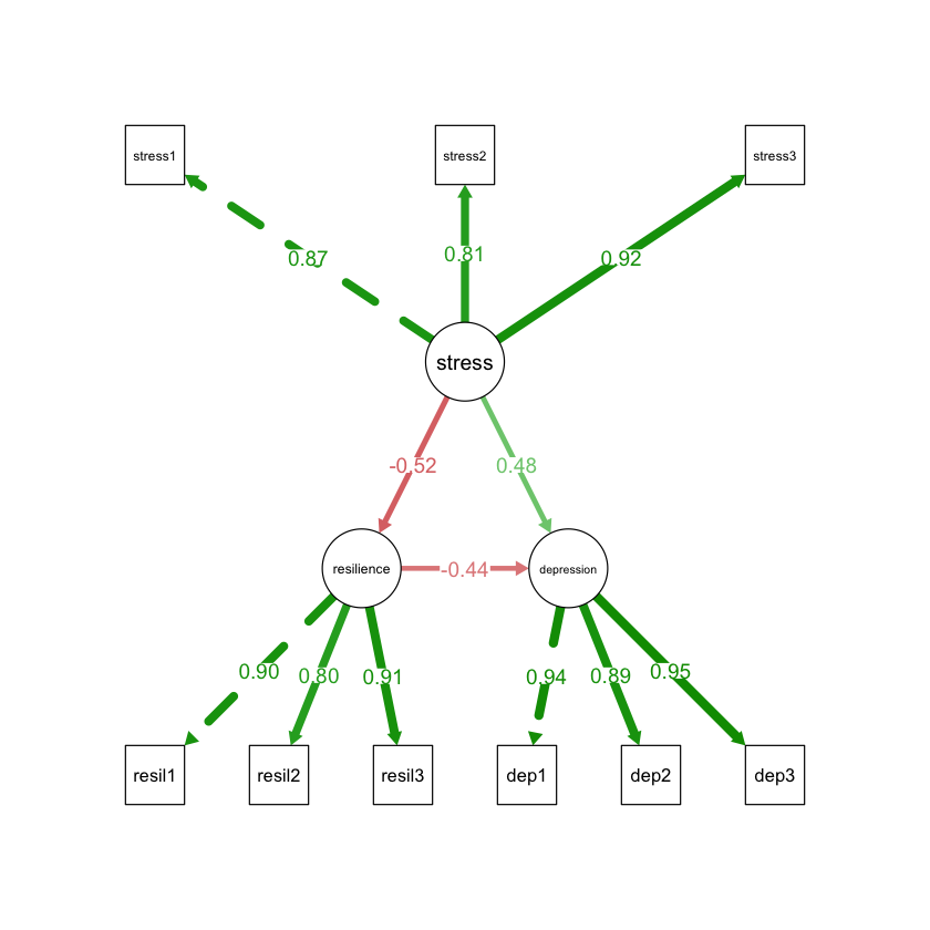
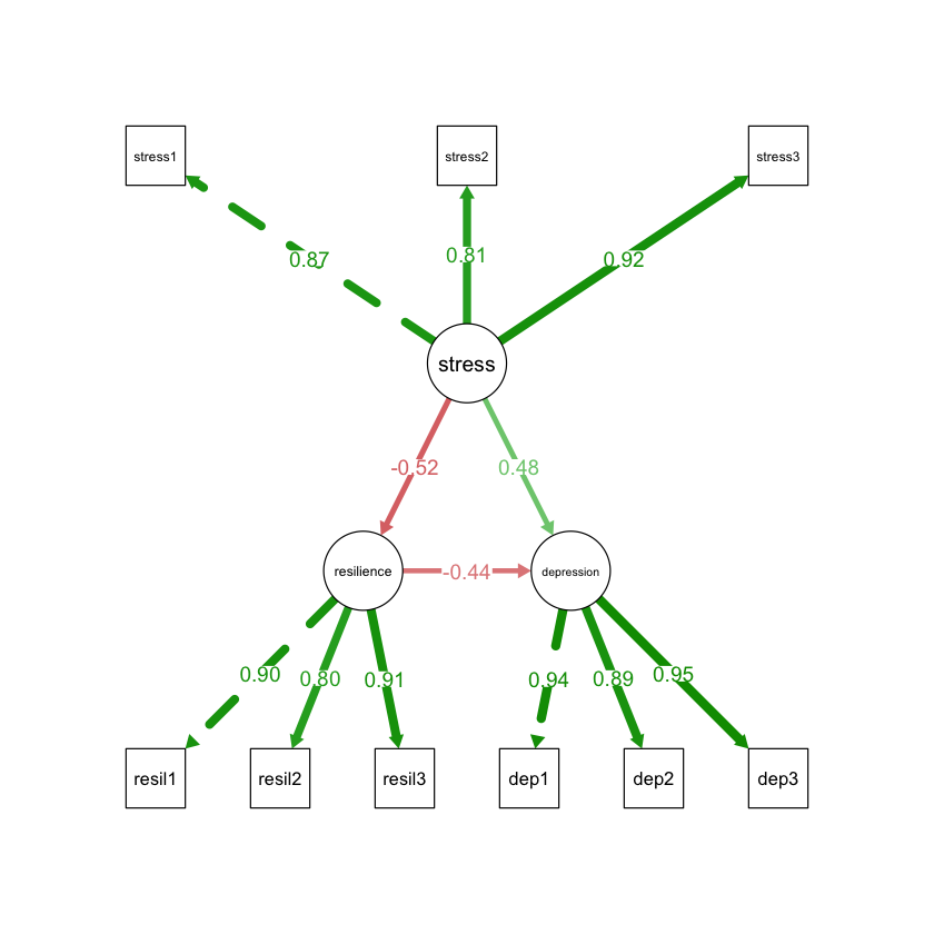
This produces a path diagram. In the diagram, circles represent latent variables, rectangles represent observed variables, arrows represent regression or measurement paths, and the numbers on the arrows are standardized coefficients.

For this fitted model, the diagram would show: stress loading onto stress1/stress2/stress3 at roughly 0.87 / 0.81 / 0.92; resilience loading onto its three indicators at roughly 0.90 / 0.80 / 0.91; depression loading onto its three indicators at roughly 0.94 / 0.89 / 0.95; a stress → resilience path around −0.52; a resilience → depression path around −0.44; and a stress → depression path around 0.48.

13 Mediation in SEM

One of the most useful applications of SEM is mediation analysis. In our example:

\[\text{Stress} \rightarrow \text{Resilience} \rightarrow \text{Depression}\]

meaning stress may affect depression indirectly, through resilience. The indirect effect is $\text{indirect} := a \times b$, where $a$ is the effect of stress on resilience and $b$ is the effect of resilience on depression. The total effect is $\text{total} := \text{direct} + \text{indirect}$.

parameterEstimates(
  fit_sem,
  standardized = TRUE
)

A lavaan.data.frame: 39 × 12
lhs	op	rhs	label	est	se	z	pvalue	ci.lower	ci.upper	std.lv	std.all
<chr>	<chr>	<chr>	<chr>	<dbl>	<dbl>	<dbl>	<dbl>	<dbl>	<dbl>	<dbl>	<dbl>
stress	=~	stress1		1.000000000	0.00000000	NA	NA	1.00000000	1.00000000	0.743305042	0.868605970
stress	=~	stress2		0.888712566	0.03965218	22.4127048	0.000000e+00	0.81099572	0.96642941	0.660584531	0.807109561
stress	=~	stress3		1.165333138	0.04332610	26.8967905	0.000000e+00	1.08041554	1.25025074	0.866197997	0.917815829
resilience	=~	resil1		1.000000000	0.00000000	NA	NA	1.00000000	1.00000000	0.771457415	0.896166093
resilience	=~	resil2		0.851920295	0.03685346	23.1164239	0.000000e+00	0.77968883	0.92415176	0.657220229	0.803459938
resilience	=~	resil3		1.123935553	0.04011596	28.0171692	0.000000e+00	1.04530972	1.20256138	0.867068417	0.905885416
depression	=~	dep1		1.000000000	0.00000000	NA	NA	1.00000000	1.00000000	1.115486326	0.939423104
depression	=~	dep2		0.852686146	0.02485828	34.3018961	0.000000e+00	0.80396481	0.90140748	0.951159737	0.891874563
depression	=~	dep3		1.146769075	0.02726355	42.0623568	0.000000e+00	1.09333350	1.20020465	1.279205223	0.950922084
resilience	~	stress	a	-0.536162652	0.04798759	-11.1729444	0.000000e+00	-0.63021660	-0.44210871	-0.516596762	-0.516596762
depression	~	resilience	b	-0.638717896	0.05641726	-11.3213206	0.000000e+00	-0.74929370	-0.52814210	-0.441729894	-0.441729894
depression	~	stress	c	0.727534488	0.05968082	12.1904241	0.000000e+00	0.61056223	0.84450674	0.484793081	0.484793081
stress1	~~	stress1		0.179796776	0.01664951	10.7989246	0.000000e+00	0.14716434	0.21242921	0.179796776	0.245523668
stress2	~~	stress2		0.233500062	0.01801124	12.9641268	0.000000e+00	0.19819867	0.26880145	0.233500062	0.348574156
stress3	~~	stress3		0.140384235	0.01830990	7.6671204	1.754152e-14	0.10449748	0.17627099	0.140384235	0.157614104
resil1	~~	resil1		0.145902412	0.01563347	9.3326929	0.000000e+00	0.11526137	0.17654346	0.145902412	0.196886334
resil2	~~	resil2		0.237165208	0.01806223	13.1304497	0.000000e+00	0.20176389	0.27256653	0.237165208	0.354452128
resil3	~~	resil3		0.164328886	0.01895948	8.6673739	0.000000e+00	0.12716899	0.20148878	0.164328886	0.179371612
dep1	~~	dep1		0.165647777	0.01695952	9.7672442	0.000000e+00	0.13240773	0.19888783	0.165647777	0.117484232
dep2	~~	dep2		0.232658848	0.01803935	12.8972957	0.000000e+00	0.19730237	0.26801533	0.232658848	0.204559764
dep3	~~	dep3		0.173267305	0.02052209	8.4429653	0.000000e+00	0.13304475	0.21348986	0.173267305	0.095747191
stress	~~	stress		0.552502385	0.04651494	11.8779564	0.000000e+00	0.46133479	0.64366999	1.000000000	1.000000000
resilience	~~	resilience		0.436318467	0.03668041	11.8951349	0.000000e+00	0.36442618	0.50821076	0.733127786	0.733127786
depression	~~	depression		0.433759482	0.03669715	11.8199764	0.000000e+00	0.36183438	0.50568458	0.348594459	0.348594459
stress1	~1			0.051164260	0.03827007	1.3369262	1.812467e-01	-0.02384370	0.12617222	0.051164260	0.059789157
stress2	~1			-0.007807425	0.03660251	-0.2133030	8.310907e-01	-0.07954703	0.06393218	-0.007807425	-0.009539199
stress3	~1			0.040657971	0.04220624	0.9633167	3.353886e-01	-0.04206473	0.12338067	0.040657971	0.043080830
resil1	~1			-0.024374481	0.03849802	-0.6331359	5.266449e-01	-0.09982922	0.05108026	-0.024374481	-0.028314698
resil2	~1			-0.011269369	0.03658152	-0.3080618	7.580353e-01	-0.08296782	0.06042908	-0.011269369	-0.013776944
resil3	~1			-0.035980507	0.04280506	-0.8405667	4.005907e-01	-0.11987688	0.04791587	-0.035980507	-0.037591286
dep1	~1			0.037102437	0.05310287	0.6986898	4.847459e-01	-0.06697728	0.14118215	0.037102437	0.031246359
dep2	~1			0.047620784	0.04769410	0.9984627	3.180550e-01	-0.04585794	0.14109951	0.047620784	0.044652611
dep3	~1			0.069974908	0.06016034	1.1631401	2.447726e-01	-0.04793719	0.18788701	0.069974908	0.052017209
stress	~1			0.000000000	0.00000000	NA	NA	0.00000000	0.00000000	0.000000000	0.000000000
resilience	~1			0.000000000	0.00000000	NA	NA	0.00000000	0.00000000	0.000000000	0.000000000
depression	~1			0.000000000	0.00000000	NA	NA	0.00000000	0.00000000	0.000000000	0.000000000
indirect	:=	a*b	indirect	0.342456681	0.04061961	8.4308214	0.000000e+00	0.26284371	0.42206965	0.228196233	0.228196233
direct	:=	c	direct	0.727534488	0.05968082	12.1904241	0.000000e+00	0.61056223	0.84450674	0.484793081	0.484793081
total	:=	c+(a*b)	total	1.069991169	0.06169700	17.3426763	0.000000e+00	0.94906726	1.19091507	0.712989314	0.712989314

The key rows of that output are the ones we already labeled in the model syntax:

Effect	Estimate	SE	z	p
indirect (`a*b`)	0.342	0.041	8.43	<.001
direct (`c`)	0.728	0.060	12.19	<.001
total (`c + a*b`)	1.070	0.062	17.34	<.001

This confirms both a direct effect of stress on depression and a meaningful indirect (mediated) effect through resilience — together summing to the total effect.

14 Bootstrapped Confidence Intervals for Indirect Effects

Indirect effects often have non-normal sampling distributions, so bootstrapping is commonly used for mediation inference instead of relying on the normal-theory z-test.

fit_sem_boot <- sem(
  model_sem,
  data = data_sem,
  se = "bootstrap",
  bootstrap = 1000,
  meanstructure = TRUE
)

parameterEstimates(
  fit_sem_boot,
  boot.ci.type = "perc",
  standardized = TRUE
)

A lavaan.data.frame: 39 × 12
lhs	op	rhs	label	est	se	z	pvalue	ci.lower	ci.upper	std.lv	std.all
<chr>	<chr>	<chr>	<chr>	<dbl>	<dbl>	<dbl>	<dbl>	<dbl>	<dbl>	<dbl>	<dbl>
stress	=~	stress1		1.000000000	0.00000000	NA	NA	1.00000000	1.00000000	0.743305042	0.868605970
stress	=~	stress2		0.888712566	0.03875278	22.9328715	0.000000e+00	0.81296490	0.96278456	0.660584531	0.807109561
stress	=~	stress3		1.165333138	0.04330515	26.9098040	0.000000e+00	1.08137123	1.25711142	0.866197997	0.917815829
resilience	=~	resil1		1.000000000	0.00000000	NA	NA	1.00000000	1.00000000	0.771457415	0.896166093
resilience	=~	resil2		0.851920295	0.03808626	22.3681820	0.000000e+00	0.77898450	0.92590202	0.657220229	0.803459938
resilience	=~	resil3		1.123935553	0.04317346	26.0330200	0.000000e+00	1.04008005	1.21317797	0.867068417	0.905885416
depression	=~	dep1		1.000000000	0.00000000	NA	NA	1.00000000	1.00000000	1.115486326	0.939423104
depression	=~	dep2		0.852686146	0.02355667	36.1972280	0.000000e+00	0.80457833	0.89658444	0.951159737	0.891874563
depression	=~	dep3		1.146769075	0.02873547	39.9077899	0.000000e+00	1.09159357	1.20370831	1.279205223	0.950922084
resilience	~	stress	a	-0.536162652	0.04772853	-11.2335886	0.000000e+00	-0.63015064	-0.44693992	-0.516596762	-0.516596762
depression	~	resilience	b	-0.638717896	0.05169940	-12.3544541	0.000000e+00	-0.74788338	-0.54120024	-0.441729894	-0.441729894
depression	~	stress	c	0.727534488	0.05869613	12.3949303	0.000000e+00	0.61975331	0.85032347	0.484793081	0.484793081
stress1	~~	stress1		0.179796776	0.01502245	11.9685414	0.000000e+00	0.14883131	0.20843282	0.179796776	0.245523668
stress2	~~	stress2		0.233500062	0.01885213	12.3858737	0.000000e+00	0.19576134	0.27184260	0.233500062	0.348574156
stress3	~~	stress3		0.140384235	0.01843239	7.6161708	2.620126e-14	0.10418247	0.17538170	0.140384235	0.157614104
resil1	~~	resil1		0.145902412	0.01595743	9.1432259	0.000000e+00	0.11363838	0.17838381	0.145902412	0.196886334
resil2	~~	resil2		0.237165208	0.01709337	13.8746937	0.000000e+00	0.20370321	0.27054419	0.237165208	0.354452128
resil3	~~	resil3		0.164328886	0.02084598	7.8830019	3.108624e-15	0.12386293	0.20364139	0.164328886	0.179371612
dep1	~~	dep1		0.165647777	0.01906716	8.6875974	0.000000e+00	0.12656908	0.20048704	0.165647777	0.117484232
dep2	~~	dep2		0.232658848	0.01764236	13.1875122	0.000000e+00	0.19903614	0.26820314	0.232658848	0.204559764
dep3	~~	dep3		0.173267305	0.02048533	8.4581171	0.000000e+00	0.13453217	0.21504703	0.173267305	0.095747191
stress	~~	stress		0.552502385	0.04695879	11.7656873	0.000000e+00	0.46231792	0.64888754	1.000000000	1.000000000
resilience	~~	resilience		0.436318467	0.03765419	11.5875151	0.000000e+00	0.36516158	0.50533324	0.733127786	0.733127786
depression	~~	depression		0.433759482	0.03872977	11.1996388	0.000000e+00	0.35791846	0.51338908	0.348594459	0.348594459
stress1	~1			0.051164260	0.03771417	1.3566322	1.748981e-01	-0.02531084	0.12307179	0.051164260	0.059789157
stress2	~1			-0.007807425	0.03691312	-0.2115081	8.324908e-01	-0.08111150	0.06529539	-0.007807425	-0.009539199
stress3	~1			0.040657971	0.04279942	0.9499654	3.421298e-01	-0.04122633	0.12437364	0.040657971	0.043080830
resil1	~1			-0.024374481	0.03766567	-0.6471272	5.175496e-01	-0.09808678	0.05658945	-0.024374481	-0.028314698
resil2	~1			-0.011269369	0.03674697	-0.3066748	7.590909e-01	-0.08130063	0.06230864	-0.011269369	-0.013776944
resil3	~1			-0.035980507	0.04224272	-0.8517564	3.943493e-01	-0.11875072	0.04734353	-0.035980507	-0.037591286
dep1	~1			0.037102437	0.05255557	0.7059658	4.802094e-01	-0.06456298	0.14260961	0.037102437	0.031246359
dep2	~1			0.047620784	0.04743160	1.0039886	3.153841e-01	-0.04997907	0.14185914	0.047620784	0.044652611
dep3	~1			0.069974908	0.05921142	1.1817807	2.372927e-01	-0.05015772	0.18235691	0.069974908	0.052017209
stress	~1			0.000000000	0.00000000	NA	NA	0.00000000	0.00000000	0.000000000	0.000000000
resilience	~1			0.000000000	0.00000000	NA	NA	0.00000000	0.00000000	0.000000000	0.000000000
depression	~1			0.000000000	0.00000000	NA	NA	0.00000000	0.00000000	0.000000000	0.000000000
indirect	:=	a*b	indirect	0.342456681	0.03929570	8.7148636	0.000000e+00	0.26652179	0.41898946	0.228196233	0.228196233
direct	:=	c	direct	0.727534488	0.05869613	12.3949303	0.000000e+00	0.61975331	0.85032347	0.484793081	0.484793081
total	:=	c+(a*b)	total	1.069991169	0.06601319	16.2087480	0.000000e+00	0.94318488	1.20050726	0.712989314	0.712989314

With 1,000 bootstrap resamples, the key structural and derived-effect estimates were essentially unchanged from the normal-theory fit, with modestly different standard errors:

Effect	Estimate	Bootstrap SE	z	p
resilience ~ stress (`a`)	−0.536	0.048	−11.23	<.001
depression ~ resilience (`b`)	−0.639	0.052	−12.35	<.001
depression ~ stress (`c`)	0.728	0.059	12.39	<.001
indirect (`a*b`)	0.342	0.039	8.71	<.001
direct (`c`)	0.728	0.059	12.39	<.001
total (`c + a*b`)	1.070	0.066	16.21	<.001

If the bootstrap confidence interval for the indirect effect does not include zero, that supports evidence for mediation — as it doesn’t here.

15 CFA Before SEM

In practice, it’s often useful to fit the measurement model alone first, before adding any structural paths.

# ------------------------------------------------------------
# 5. Confirmatory Factor Analysis first
# ------------------------------------------------------------
model_cfa <- '
  stress     =~ stress1 + stress2 + stress3
  resilience =~ resil1 + resil2 + resil3
  depression =~ dep1 + dep2 + dep3
'

fit_cfa <- cfa(
  model_cfa,
  data = data_sem,
  meanstructure = TRUE
)

summary(
  fit_cfa,
  fit.measures = TRUE,
  standardized = TRUE
)

$header

$lavaan.version: '0.7-2'
$sam.approach: FALSE
$optim.method: 'nlminb'
$optim.iterations: 43
$optim.converged: TRUE

$optim

$estimator

'ML'

$estimator.args

$optim.method

'nlminb'

$npar

$eq.constraints

FALSE

$nrow.ceq.jac

$nrow.cin.jac

$nrow.con.jac

$con.jac.rank

$data

$ngroups: 1
$nobs: 500

$test

$standard =

$test: 'standard'
$stat: 39.5933180434271
$stat.group: 39.5933180434271
$df: 24
$refdistr: 'chisq'
$pvalue: 0.0236381876165893

$fit

npar: 30
fmin: 0.0395933180434271
chisq: 39.5933180434271
df: 24
pvalue: 0.0236381876165893
baseline.chisq: 4010.69045035666
baseline.df: 36
baseline.pvalue: 0
cfi: 0.996076847181388
tli: 0.994115270772082
logl: -4261.75022147891
unrestricted.logl: -4241.95356245719
aic: 8583.50044295782
bic: 8709.93868591049
ntotal: 500
bic2: 8614.71683163813
rmsea: 0.0360477900887918
rmsea.ci.lower: 0.0133206537566257
rmsea.ci.upper: 0.0554785467014227
rmsea.ci.level: 0.9
rmsea.pvalue: 0.872609329435695
rmsea.close.h0: 0.05
rmsea.notclose.pvalue: 2.92071859397014e-05
rmsea.notclose.h0: 0.08
srmr: 0.0195584666176241
gfi: 0.994230150253581
gfi.ci.lower: 0.98528160224032
gfi.ci.upper: 0.999811176769756
gfi.ci.level: 0.9

$pe

A data.frame: 33 × 10
	lhs	op	rhs	exo	est	se	z	pvalue	std.lv	std.all
	<chr>	<chr>	<chr>	<int>	<dbl>	<dbl>	<dbl>	<dbl>	<dbl>	<dbl>
1	stress	=~	stress1	0	1.000000000	0.00000000	NA	NA	0.743304970	0.86860600
2	stress	=~	stress2	0	0.888712491	0.03965218	22.4127035	0.000000e+00	0.660584412	0.80710955
3	stress	=~	stress3	0	1.165332895	0.04332610	26.8967848	0.000000e+00	0.866197733	0.91781573
4	resilience	=~	resil1	0	1.000000000	0.00000000	NA	NA	0.771457341	0.89616610
5	resilience	=~	resil2	0	0.851920122	0.03685347	23.1164167	0.000000e+00	0.657220032	0.80345979
6	resilience	=~	resil3	0	1.123935775	0.04011596	28.0171702	0.000000e+00	0.867068504	0.90588546
7	depression	=~	dep1	0	1.000000000	0.00000000	NA	NA	1.115486234	0.93942308
8	depression	=~	dep2	0	0.852686291	0.02485828	34.3018972	0.000000e+00	0.951159819	0.89187460
9	depression	=~	dep3	0	1.146769204	0.02726356	42.0623465	0.000000e+00	1.279205260	0.95092205
10	stress1	~~	stress1	0	0.179796686	0.01664951	10.7989206	0.000000e+00	0.179796686	0.24552361
11	stress2	~~	stress2	0	0.233499998	0.01801124	12.9641256	0.000000e+00	0.233499998	0.34857418
12	stress3	~~	stress3	0	0.140384332	0.01830990	7.6671251	1.754152e-14	0.140384332	0.15761428
13	resil1	~~	resil1	0	0.145902374	0.01563347	9.3326916	0.000000e+00	0.145902374	0.19688632
14	resil2	~~	resil2	0	0.237165314	0.01806223	13.1304527	0.000000e+00	0.237165314	0.35445237
15	resil3	~~	resil3	0	0.164328836	0.01895948	8.6673701	0.000000e+00	0.164328836	0.17937154
16	dep1	~~	dep1	0	0.165647815	0.01695952	9.7672450	0.000000e+00	0.165647815	0.11748427
17	dep2	~~	dep2	0	0.232658800	0.01803935	12.8972935	0.000000e+00	0.232658800	0.20455970
18	dep3	~~	dep3	0	0.173267425	0.02052210	8.4429675	0.000000e+00	0.173267425	0.09574725
19	stress	~~	stress	0	0.552502279	0.04651493	11.8779567	0.000000e+00	1.000000000	1.00000000
20	resilience	~~	resilience	0	0.595146428	0.04765206	12.4894168	0.000000e+00	1.000000000	1.00000000
21	depression	~~	depression	0	1.244309537	0.08955462	13.8944197	0.000000e+00	1.000000000	1.00000000
22	stress	~~	resilience	0	-0.296230974	0.03244527	-9.1301739	0.000000e+00	-0.516596565	-0.51659657
23	stress	~~	depression	0	0.591172397	0.05054565	11.6958112	0.000000e+00	0.712989110	0.71298911
24	resilience	~~	depression	0	-0.595649001	0.05120134	-11.6334641	0.000000e+00	-0.692172414	-0.69217241
25	stress1	~1		0	0.051164260	0.03827007	1.3369264	1.812467e-01	0.051164260	0.05978917
26	stress2	~1		0	-0.007807425	0.03660251	-0.2133030	8.310906e-01	-0.007807425	-0.00953920
27	stress3	~1		0	0.040657971	0.04220623	0.9633169	3.353885e-01	0.040657971	0.04308084
28	resil1	~1		0	-0.024374481	0.03849802	-0.6331360	5.266449e-01	-0.024374481	-0.02831470
29	resil2	~1		0	-0.011269369	0.03658151	-0.3080619	7.580353e-01	-0.011269369	-0.01377695
30	resil3	~1		0	-0.035980507	0.04280506	-0.8405667	4.005907e-01	-0.035980507	-0.03759128
31	dep1	~1		0	0.037102437	0.05310287	0.6986899	4.847459e-01	0.037102437	0.03124636
32	dep2	~1		0	0.047620784	0.04769410	0.9984627	3.180550e-01	0.047620784	0.04465261
33	dep3	~1		0	0.069974908	0.06016034	1.1631401	2.447727e-01	0.069974908	0.05201721

This CFA-only fit lets all three latent factors freely covary (rather than imposing the directional structural paths), and shows essentially identical fit to the full SEM: $\chi^2(24) = 39.59$, $p = 0.024$, CFI = 0.996, TLI = 0.994, RMSEA = 0.036, SRMR = 0.020 — and factor loadings matching those from the full model. That agreement is a good sign: it means the structural paths we added aren’t distorting the measurement model, and the latent constructs are well identified on their own.

This checks whether the measurement structure is reasonable before adding structural paths. A good general workflow:

Check the measurement model using CFA.
Check reliability and factor loadings.
Fit the full SEM model.
Interpret direct, indirect, and total effects.
Report model fit and standardized estimates.

16 SEM Versus Regression

Regression and SEM are related, but SEM is more general.

Feature	Regression	SEM
Observed variables	Yes	Yes
Latent variables	No	Yes
Multiple outcomes	Limited	Yes
Measurement error	Usually ignored	Explicitly modeled
Mediation	Possible	Natural framework
Model fit	Usually not covariance-based	Central part of SEM
Theory testing	Limited	Strong

Regression is often enough when the research question is simple and all variables are directly observed. SEM is worth reaching for when constructs are latent, measurement error matters, several equations are needed at once, mediation is central to the question, or the theoretical structure itself is part of what’s being tested.

17 Assumptions of SEM

SEM rests on assumptions that should be considered carefully.

17.1 Correct Model Specification

The model should be theoretically justified. SEM can test whether a model is consistent with the data, but it cannot prove that the model is true — a good-fitting model is not necessarily the only good-fitting model.

17.2 Adequate Sample Size

SEM usually requires moderate to large sample sizes. There’s no single universal rule, but small samples can lead to unstable estimates, convergence problems, or unreliable fit indices.

17.3 Multivariate Normality

Classical SEM often assumes multivariate normality, especially under maximum likelihood estimation. If variables are non-normal, robust estimators can be used instead:

fit_robust <- sem(
  model_sem,
  data = data_sem,
  estimator = "MLR",
  meanstructure = TRUE
)

summary(
  fit_robust,
  fit.measures = TRUE,
  standardized = TRUE
)

lavaan NOTE:  
   Standard errors and confidence intervals of the (nonlinear) defined (:=) 
   parameters are based on the first-order delta method; for strongly 
   nonlinear definitions, se.def = "mc" (Monte Carlo) or se = "bootstrap" may 
   be more accurate.

$header

$lavaan.version: '0.7-2'
$sam.approach: FALSE
$optim.method: 'nlminb'
$optim.iterations: 34
$optim.converged: TRUE

$optim

$estimator

'ML'

$estimator.args

$optim.method

'nlminb'

$npar

$eq.constraints

FALSE

$nrow.ceq.jac

$nrow.cin.jac

$nrow.con.jac

$con.jac.rank

$data

$ngroups: 1
$nobs: 500

$test

$standard

$test: 'standard'
$stat: 39.5933180430763
$stat.group: 39.5933180430763
$df: 24
$refdistr: 'chisq'
$pvalue: 0.023638187618621

$yuan.bentler.mplus

$test: 'yuan.bentler.mplus'
$stat: 39.1136150602653
$stat.group: 39.1136150602653
$df: 24
$pvalue: 0.0265687152629294
$scaling.factor: 1.01226434790218
$scaling.factor.h1: 1.00598789331404
$scaling.factor.h0: 1.00096672964353
$label: 'Yuan-Bentler correction (Mplus variant)'
$trace.UGamma: 24.2943443496523
$trace.UGamma2: <NA>
$scaled.test.stat: 39.5933180430763
$scaled.test: 'standard'

$fit

npar: 30
fmin: 0.0395933180430763
chisq: 39.5933180430763
df: 24
pvalue: 0.023638187618621
chisq.scaled: 39.1136150602653
df.scaled: 24
pvalue.scaled: 0.0265687152629294
chisq.scaling.factor: 1.01226434790218
baseline.chisq: 4010.69045035666
baseline.df: 36
baseline.pvalue: 0
baseline.chisq.scaled: 3976.21261425848
baseline.df.scaled: 36
baseline.pvalue.scaled: 0
baseline.chisq.scaling.factor: 1.00867102427434
cfi: 0.996076847181476
tli: 0.994115270772214
cfi.scaled: 0.996164264079158
tli.scaled: 0.994246396118737
cfi.robust: 0.99615059952433
tli.robust: 0.994225899286495
logl: -4261.75022147873
unrestricted.logl: -4241.95356245719
aic: 8583.50044295747
bic: 8709.93868591013
ntotal: 500
bic2: 8614.71683163778
scaling.factor.h1: 1.00598789331404
scaling.factor.h0: 1.00096672964353
rmsea: 0.0360477900883863
rmsea.ci.lower: 0.0133206537558792
rmsea.ci.upper: 0.0554785467010791
rmsea.ci.level: 0.9
rmsea.pvalue: 0.872609329442447
rmsea.close.h0: 0.05
rmsea.notclose.pvalue: 2.92071859358351e-05
rmsea.notclose.h0: 0.08
rmsea.scaled: 0.0354889831030529
rmsea.ci.lower.scaled: 0.0124583878620228
rmsea.ci.upper.scaled: 0.0548896214404359
rmsea.pvalue.scaled: 0.88324809904409
rmsea.notclose.pvalue.scaled: 2.18002882029145e-05
rmsea.robust: 0.0357059445254148
rmsea.ci.lower.robust: 0.0123349424481562
rmsea.ci.upper.robust: 0.0553426342690385
rmsea.pvalue.robust: 0.876068710519012
rmsea.notclose.pvalue.robust: 2.98978644814493e-05
srmr: 0.0195584346342506
gfi: 0.994230146309336
gfi.ci.lower: 0.985281597136529
gfi.ci.upper: 0.999811174122434
gfi.ci.level: 0.9
gfi.robust: 0.994359477575713
gfi.ci.lower.robust: 0.985362374926487
gfi.ci.upper.robust: 0.999942565997681

$pe

A data.frame: 36 × 11
	lhs	op	rhs	label	exo	est	se	z	pvalue	std.lv	std.all
	<chr>	<chr>	<chr>	<chr>	<int>	<dbl>	<dbl>	<dbl>	<dbl>	<dbl>	<dbl>
1	stress	=~	stress1		0	1.000000000	0.00000000	NA	NA	0.743305042	0.868605970
2	stress	=~	stress2		0	0.888712566	0.03942880	22.5396804	0.000000e+00	0.660584531	0.807109561
3	stress	=~	stress3		0	1.165333138	0.04482736	25.9960266	0.000000e+00	0.866197997	0.917815829
4	resilience	=~	resil1		0	1.000000000	0.00000000	NA	NA	0.771457415	0.896166093
5	resilience	=~	resil2		0	0.851920295	0.03803463	22.3985404	0.000000e+00	0.657220229	0.803459938
6	resilience	=~	resil3		0	1.123935553	0.04081111	27.5399390	0.000000e+00	0.867068417	0.905885416
7	depression	=~	dep1		0	1.000000000	0.00000000	NA	NA	1.115486326	0.939423104
8	depression	=~	dep2		0	0.852686146	0.02411456	35.3598025	0.000000e+00	0.951159737	0.891874563
9	depression	=~	dep3		0	1.146769075	0.02812917	40.7679698	0.000000e+00	1.279205223	0.950922084
10	resilience	~	stress	a	0	-0.536162652	0.04762429	-11.2581761	0.000000e+00	-0.516596762	-0.516596762
11	depression	~	resilience	b	0	-0.638717896	0.05328262	-11.9873592	0.000000e+00	-0.441729894	-0.441729894
12	depression	~	stress	c	0	0.727534488	0.05931887	12.2648068	0.000000e+00	0.484793081	0.484793081
13	stress1	~~	stress1		0	0.179796776	0.01502218	11.9687500	0.000000e+00	0.179796776	0.245523668
14	stress2	~~	stress2		0	0.233500062	0.01873282	12.4647549	0.000000e+00	0.233500062	0.348574156
15	stress3	~~	stress3		0	0.140384235	0.01809214	7.7594060	8.437695e-15	0.140384235	0.157614104
16	resil1	~~	resil1		0	0.145902412	0.01518287	9.6096700	0.000000e+00	0.145902412	0.196886334
17	resil2	~~	resil2		0	0.237165208	0.01635885	14.4976666	0.000000e+00	0.237165208	0.354452128
18	resil3	~~	resil3		0	0.164328886	0.02044476	8.0377007	8.881784e-16	0.164328886	0.179371612
19	dep1	~~	dep1		0	0.165647777	0.01833613	9.0339534	0.000000e+00	0.165647777	0.117484232
20	dep2	~~	dep2		0	0.232658848	0.01754117	13.2635869	0.000000e+00	0.232658848	0.204559764
21	dep3	~~	dep3		0	0.173267305	0.02076417	8.3445350	0.000000e+00	0.173267305	0.095747191
22	stress	~~	stress		0	0.552502385	0.04624425	11.9474836	0.000000e+00	1.000000000	1.000000000
23	resilience	~~	resilience		0	0.436318467	0.03737519	11.6740140	0.000000e+00	0.733127786	0.733127786
24	depression	~~	depression		0	0.433759482	0.03861860	11.2318795	0.000000e+00	0.348594459	0.348594459
25	stress1	~1			0	0.051164260	0.03827007	1.3369262	1.812467e-01	0.051164260	0.059789157
26	stress2	~1			0	-0.007807425	0.03660251	-0.2133030	8.310907e-01	-0.007807425	-0.009539199
27	stress3	~1			0	0.040657971	0.04220624	0.9633167	3.353886e-01	0.040657971	0.043080830
28	resil1	~1			0	-0.024374481	0.03849803	-0.6331359	5.266449e-01	-0.024374481	-0.028314698
29	resil2	~1			0	-0.011269369	0.03658152	-0.3080618	7.580353e-01	-0.011269369	-0.013776944
30	resil3	~1			0	-0.035980507	0.04280506	-0.8405667	4.005907e-01	-0.035980507	-0.037591286
31	dep1	~1			0	0.037102437	0.05310288	0.6986898	4.847459e-01	0.037102437	0.031246359
32	dep2	~1			0	0.047620784	0.04769411	0.9984627	3.180551e-01	0.047620784	0.044652611
33	dep3	~1			0	0.069974908	0.06016035	1.1631401	2.447727e-01	0.069974908	0.052017209
37	indirect	:=	a*b	indirect	0	0.342456681	0.04001743	8.5576878	0.000000e+00	0.228196233	0.228196233
38	direct	:=	c	direct	0	0.727534488	0.05931887	12.2648068	0.000000e+00	0.484793081	0.484793081
39	total	:=	c+(a*b)	total	0	1.069991169	0.06527865	16.3911355	0.000000e+00	0.712989314	0.712989314

MLR provides robust (sandwich-type) standard errors and a robust test statistic. In this dataset it changes very little — the raw chi-square is identical (39.593, df = 24), with a Yuan-Bentler scaled chi-square of 39.11 (scaling factor ≈ 1.01) and a robust RMSEA of 0.036 — reassuring, since it suggests the normal-theory results weren’t being distorted by non-normality in the simulated data.

17.4 Missing Data

SEM can handle missing data using full information maximum likelihood (FIML):

fit_missing <- sem(
  model_sem,
  data = data_sem,
  missing = "fiml",
  meanstructure = TRUE
)

This is generally preferable to simply deleting all rows with missing values (listwise deletion), assuming the missing-data mechanism is appropriate for FIML (missing at random).

18 Modification Indices

Modification indices suggest possible model changes that might improve fit.

modindices(
  fit_sem,
  sort = TRUE,
  minimum.value = 10
)

A lavaan.data.frame: 2 × 8
	lhs	op	rhs	mi	epc	sepc.lv	sepc.all	sepc.nox
	<chr>	<chr>	<chr>	<dbl>	<dbl>	<dbl>	<dbl>	<dbl>
66	stress2	~~	stress3	15.32568	-0.08218576	-0.08218576	-0.4539352	-0.4539352
52	depression	=~	stress1	15.31238	-0.13934818	-0.15544099	-0.1816441	-0.1816441

lhs	op	rhs	mi	epc	sepc.all
stress2		stress3	15.33	−0.082	−0.454
depression	=~	stress1	15.31	−0.139	−0.182

Both suggested modifications clear the conventional threshold of 10, but that doesn’t mean either should automatically be added.

Modification indices should be used cautiously. Don’t blindly add paths just because they improve model fit — every added path should have theoretical justification. Otherwise the model becomes data-driven and may not replicate.

19 Reporting SEM Results

A clear SEM report should include: the theoretical model, a description of the observed indicators, the estimator used, the sample size, model fit indices, standardized factor loadings, structural path coefficients, direct/indirect/total effects if mediation is tested, any model modifications, and limitations.

Example reporting paragraph:

We fitted a structural equation model to examine whether resilience mediated the association between stress and depression. Stress, resilience, and depression were modeled as latent variables, each measured by three observed indicators. The model showed acceptable fit according to CFI, TLI, RMSEA, and SRMR. Standardized path estimates indicated that higher stress was associated with lower resilience, and higher resilience was associated with lower depression. The indirect effect from stress to depression through resilience was estimated using bootstrapped confidence intervals.

20 Common Mistakes in SEM

Mistake 1: Treating SEM as causal proof. SEM can represent causal hypotheses, but it does not prove causality by itself. Causal interpretation depends on study design, theory, temporal ordering, confounding control, and the underlying assumptions.

Mistake 2: Ignoring the measurement model. If the latent variables are poorly measured, the structural paths built on top of them may not be meaningful.

Mistake 3: Chasing fit indices. Good fit indices do not guarantee that the model is scientifically meaningful.

Mistake 4: Overfitting with modification indices. Adding many paths based only on modification indices can make the model fit the current dataset while failing to replicate in future ones.

Mistake 5: Reporting only p-values. SEM results should include effect sizes, standardized estimates, confidence intervals, and model fit indices — not p-values alone.

21 Full R Code in One Block

# ============================================================
# Full SEM Tutorial Script
# ============================================================

library(lavaan)
library(semPlot)
library(MASS)

set.seed(123)

n <- 500
stress_latent <- rnorm(n, 0, 1)
resilience_latent <- -0.5 * stress_latent + rnorm(n, 0, 0.8)
depression_latent <- 0.6 * stress_latent -
  0.7 * resilience_latent +
  rnorm(n, 0, 0.8)

data_sem <- data.frame(
  stress1 = 0.8 * stress_latent + rnorm(n, 0, 0.4),
  stress2 = 0.7 * stress_latent + rnorm(n, 0, 0.5),
  stress3 = 0.9 * stress_latent + rnorm(n, 0, 0.4),
  resil1  = 0.8 * resilience_latent + rnorm(n, 0, 0.4),
  resil2  = 0.7 * resilience_latent + rnorm(n, 0, 0.5),
  resil3  = 0.9 * resilience_latent + rnorm(n, 0, 0.4),
  dep1    = 0.8 * depression_latent + rnorm(n, 0, 0.4),
  dep2    = 0.7 * depression_latent + rnorm(n, 0, 0.5),
  dep3    = 0.9 * depression_latent + rnorm(n, 0, 0.4)
)

model_sem <- '
  # Measurement model
  stress     =~ stress1 + stress2 + stress3
  resilience =~ resil1 + resil2 + resil3
  depression =~ dep1 + dep2 + dep3

  # Structural model
  resilience ~ a * stress
  depression ~ b * resilience + c * stress

  # Effects
  indirect := a * b
  direct   := c
  total    := c + (a * b)
'

fit_sem <- sem(
  model_sem,
  data = data_sem,
  meanstructure = TRUE
)

summary(
  fit_sem,
  fit.measures = TRUE,
  standardized = TRUE,
  rsquare = TRUE
)

fitMeasures(
  fit_sem,
  c("chisq", "df", "pvalue", "cfi", "tli", "rmsea", "srmr")
)

parameterEstimates(
  fit_sem,
  standardized = TRUE
)

semPaths(
  fit_sem,
  what = "std",
  layout = "tree",
  edge.label.cex = 1.0,
  sizeMan = 6,
  sizeLat = 8,
  residuals = FALSE,
  intercepts = FALSE,
  nCharNodes = 0
)

fit_sem_boot <- sem(
  model_sem,
  data = data_sem,
  se = "bootstrap",
  bootstrap = 1000,
  meanstructure = TRUE
)

parameterEstimates(
  fit_sem_boot,
  boot.ci.type = "perc",
  standardized = TRUE
)

lavaan NOTE:  
   Standard errors and confidence intervals of the (nonlinear) defined (:=) 
   parameters are based on the first-order delta method; for strongly 
   nonlinear definitions, se.def = "mc" (Monte Carlo) or se = "bootstrap" may 
   be more accurate.

$header

$lavaan.version: '0.7-2'
$sam.approach: FALSE
$optim.method: 'nlminb'
$optim.iterations: 34
$optim.converged: TRUE

$optim

$estimator

'ML'

$estimator.args

$optim.method

'nlminb'

$npar

$eq.constraints

FALSE

$nrow.ceq.jac

$nrow.cin.jac

$nrow.con.jac

$con.jac.rank

$data

$ngroups: 1
$nobs: 500

$test

$standard =

$test: 'standard'
$stat: 39.5933180430763
$stat.group: 39.5933180430763
$df: 24
$refdistr: 'chisq'
$pvalue: 0.023638187618621

$fit

npar: 30
fmin: 0.0395933180430763
chisq: 39.5933180430763
df: 24
pvalue: 0.023638187618621
baseline.chisq: 4010.69045035666
baseline.df: 36
baseline.pvalue: 0
cfi: 0.996076847181476
tli: 0.994115270772214
logl: -4261.75022147873
unrestricted.logl: -4241.95356245719
aic: 8583.50044295747
bic: 8709.93868591013
ntotal: 500
bic2: 8614.71683163778
rmsea: 0.0360477900883863
rmsea.ci.lower: 0.0133206537558792
rmsea.ci.upper: 0.0554785467010791
rmsea.ci.level: 0.9
rmsea.pvalue: 0.872609329442447
rmsea.close.h0: 0.05
rmsea.notclose.pvalue: 2.92071859358351e-05
rmsea.notclose.h0: 0.08
srmr: 0.0195584346342506
gfi: 0.994230146309336
gfi.ci.lower: 0.985281597136529
gfi.ci.upper: 0.999811174122434
gfi.ci.level: 0.9

$pe

A data.frame: 47 × 11
	lhs	op	rhs	label	exo	est	se	z	pvalue	std.lv	std.all
	<chr>	<chr>	<chr>	<chr>	<int>	<dbl>	<dbl>	<dbl>	<dbl>	<dbl>	<dbl>
1	stress	=~	stress1		0	1.000000000	0.00000000	NA	NA	0.743305042	0.868605970
2	stress	=~	stress2		0	0.888712566	0.03965218	22.4127048	0.000000e+00	0.660584531	0.807109561
3	stress	=~	stress3		0	1.165333138	0.04332610	26.8967905	0.000000e+00	0.866197997	0.917815829
4	resilience	=~	resil1		0	1.000000000	0.00000000	NA	NA	0.771457415	0.896166093
5	resilience	=~	resil2		0	0.851920295	0.03685346	23.1164239	0.000000e+00	0.657220229	0.803459938
6	resilience	=~	resil3		0	1.123935553	0.04011596	28.0171692	0.000000e+00	0.867068417	0.905885416
7	depression	=~	dep1		0	1.000000000	0.00000000	NA	NA	1.115486326	0.939423104
8	depression	=~	dep2		0	0.852686146	0.02485828	34.3018961	0.000000e+00	0.951159737	0.891874563
9	depression	=~	dep3		0	1.146769075	0.02726355	42.0623568	0.000000e+00	1.279205223	0.950922084
10	resilience	~	stress	a	0	-0.536162652	0.04798759	-11.1729444	0.000000e+00	-0.516596762	-0.516596762
11	depression	~	resilience	b	0	-0.638717896	0.05641726	-11.3213206	0.000000e+00	-0.441729894	-0.441729894
12	depression	~	stress	c	0	0.727534488	0.05968082	12.1904241	0.000000e+00	0.484793081	0.484793081
13	stress1	~~	stress1		0	0.179796776	0.01664951	10.7989246	0.000000e+00	0.179796776	0.245523668
14	stress2	~~	stress2		0	0.233500062	0.01801124	12.9641268	0.000000e+00	0.233500062	0.348574156
15	stress3	~~	stress3		0	0.140384235	0.01830990	7.6671204	1.754152e-14	0.140384235	0.157614104
16	resil1	~~	resil1		0	0.145902412	0.01563347	9.3326929	0.000000e+00	0.145902412	0.196886334
17	resil2	~~	resil2		0	0.237165208	0.01806223	13.1304497	0.000000e+00	0.237165208	0.354452128
18	resil3	~~	resil3		0	0.164328886	0.01895948	8.6673739	0.000000e+00	0.164328886	0.179371612
19	dep1	~~	dep1		0	0.165647777	0.01695952	9.7672442	0.000000e+00	0.165647777	0.117484232
20	dep2	~~	dep2		0	0.232658848	0.01803935	12.8972957	0.000000e+00	0.232658848	0.204559764
21	dep3	~~	dep3		0	0.173267305	0.02052209	8.4429653	0.000000e+00	0.173267305	0.095747191
22	stress	~~	stress		0	0.552502385	0.04651494	11.8779564	0.000000e+00	1.000000000	1.000000000
23	resilience	~~	resilience		0	0.436318467	0.03668041	11.8951349	0.000000e+00	0.733127786	0.733127786
24	depression	~~	depression		0	0.433759482	0.03669715	11.8199764	0.000000e+00	0.348594459	0.348594459
25	stress1	~1			0	0.051164260	0.03827007	1.3369262	1.812467e-01	0.051164260	0.059789157
26	stress2	~1			0	-0.007807425	0.03660251	-0.2133030	8.310907e-01	-0.007807425	-0.009539199
27	stress3	~1			0	0.040657971	0.04220624	0.9633167	3.353886e-01	0.040657971	0.043080830
28	resil1	~1			0	-0.024374481	0.03849802	-0.6331359	5.266449e-01	-0.024374481	-0.028314698
29	resil2	~1			0	-0.011269369	0.03658152	-0.3080618	7.580353e-01	-0.011269369	-0.013776944
30	resil3	~1			0	-0.035980507	0.04280506	-0.8405667	4.005907e-01	-0.035980507	-0.037591286
31	dep1	~1			0	0.037102437	0.05310287	0.6986898	4.847459e-01	0.037102437	0.031246359
32	dep2	~1			0	0.047620784	0.04769410	0.9984627	3.180550e-01	0.047620784	0.044652611
33	dep3	~1			0	0.069974908	0.06016034	1.1631401	2.447726e-01	0.069974908	0.052017209
37	indirect	:=	a*b	indirect	0	0.342456681	0.04061961	8.4308214	0.000000e+00	0.228196233	0.228196233
38	direct	:=	c	direct	0	0.727534488	0.05968082	12.1904241	0.000000e+00	0.484793081	0.484793081
39	total	:=	c+(a*b)	total	0	1.069991169	0.06169700	17.3426763	0.000000e+00	0.712989314	0.712989314
40	stress1	r2	stress1		0	0.754476332	NA	NA	NA	NA	NA
41	stress2	r2	stress2		0	0.651425844	NA	NA	NA	NA	NA
42	stress3	r2	stress3		0	0.842385896	NA	NA	NA	NA	NA
43	resil1	r2	resil1		0	0.803113666	NA	NA	NA	NA	NA
44	resil2	r2	resil2		0	0.645547872	NA	NA	NA	NA	NA
45	resil3	r2	resil3		0	0.820628388	NA	NA	NA	NA	NA
46	dep1	r2	dep1		0	0.882515768	NA	NA	NA	NA	NA
47	dep2	r2	dep2		0	0.795440236	NA	NA	NA	NA	NA
48	dep3	r2	dep3		0	0.904252809	NA	NA	NA	NA	NA
49	resilience	r2	resilience		0	0.266872214	NA	NA	NA	NA	NA
50	depression	r2	depression		0	0.651405541	NA	NA	NA	NA	NA

chisq: 39.5933180430763
df: 24
pvalue: 0.023638187618621
cfi: 0.996076847181476
tli: 0.994115270772214
rmsea: 0.0360477900883863
srmr: 0.0195584346342506

A lavaan.data.frame: 39 × 12
lhs	op	rhs	label	est	se	z	pvalue	ci.lower	ci.upper	std.lv	std.all
<chr>	<chr>	<chr>	<chr>	<dbl>	<dbl>	<dbl>	<dbl>	<dbl>	<dbl>	<dbl>	<dbl>
stress	=~	stress1		1.000000000	0.00000000	NA	NA	1.00000000	1.00000000	0.743305042	0.868605970
stress	=~	stress2		0.888712566	0.03965218	22.4127048	0.000000e+00	0.81099572	0.96642941	0.660584531	0.807109561
stress	=~	stress3		1.165333138	0.04332610	26.8967905	0.000000e+00	1.08041554	1.25025074	0.866197997	0.917815829
resilience	=~	resil1		1.000000000	0.00000000	NA	NA	1.00000000	1.00000000	0.771457415	0.896166093
resilience	=~	resil2		0.851920295	0.03685346	23.1164239	0.000000e+00	0.77968883	0.92415176	0.657220229	0.803459938
resilience	=~	resil3		1.123935553	0.04011596	28.0171692	0.000000e+00	1.04530972	1.20256138	0.867068417	0.905885416
depression	=~	dep1		1.000000000	0.00000000	NA	NA	1.00000000	1.00000000	1.115486326	0.939423104
depression	=~	dep2		0.852686146	0.02485828	34.3018961	0.000000e+00	0.80396481	0.90140748	0.951159737	0.891874563
depression	=~	dep3		1.146769075	0.02726355	42.0623568	0.000000e+00	1.09333350	1.20020465	1.279205223	0.950922084
resilience	~	stress	a	-0.536162652	0.04798759	-11.1729444	0.000000e+00	-0.63021660	-0.44210871	-0.516596762	-0.516596762
depression	~	resilience	b	-0.638717896	0.05641726	-11.3213206	0.000000e+00	-0.74929370	-0.52814210	-0.441729894	-0.441729894
depression	~	stress	c	0.727534488	0.05968082	12.1904241	0.000000e+00	0.61056223	0.84450674	0.484793081	0.484793081
stress1	~~	stress1		0.179796776	0.01664951	10.7989246	0.000000e+00	0.14716434	0.21242921	0.179796776	0.245523668
stress2	~~	stress2		0.233500062	0.01801124	12.9641268	0.000000e+00	0.19819867	0.26880145	0.233500062	0.348574156
stress3	~~	stress3		0.140384235	0.01830990	7.6671204	1.754152e-14	0.10449748	0.17627099	0.140384235	0.157614104
resil1	~~	resil1		0.145902412	0.01563347	9.3326929	0.000000e+00	0.11526137	0.17654346	0.145902412	0.196886334
resil2	~~	resil2		0.237165208	0.01806223	13.1304497	0.000000e+00	0.20176389	0.27256653	0.237165208	0.354452128
resil3	~~	resil3		0.164328886	0.01895948	8.6673739	0.000000e+00	0.12716899	0.20148878	0.164328886	0.179371612
dep1	~~	dep1		0.165647777	0.01695952	9.7672442	0.000000e+00	0.13240773	0.19888783	0.165647777	0.117484232
dep2	~~	dep2		0.232658848	0.01803935	12.8972957	0.000000e+00	0.19730237	0.26801533	0.232658848	0.204559764
dep3	~~	dep3		0.173267305	0.02052209	8.4429653	0.000000e+00	0.13304475	0.21348986	0.173267305	0.095747191
stress	~~	stress		0.552502385	0.04651494	11.8779564	0.000000e+00	0.46133479	0.64366999	1.000000000	1.000000000
resilience	~~	resilience		0.436318467	0.03668041	11.8951349	0.000000e+00	0.36442618	0.50821076	0.733127786	0.733127786
depression	~~	depression		0.433759482	0.03669715	11.8199764	0.000000e+00	0.36183438	0.50568458	0.348594459	0.348594459
stress1	~1			0.051164260	0.03827007	1.3369262	1.812467e-01	-0.02384370	0.12617222	0.051164260	0.059789157
stress2	~1			-0.007807425	0.03660251	-0.2133030	8.310907e-01	-0.07954703	0.06393218	-0.007807425	-0.009539199
stress3	~1			0.040657971	0.04220624	0.9633167	3.353886e-01	-0.04206473	0.12338067	0.040657971	0.043080830
resil1	~1			-0.024374481	0.03849802	-0.6331359	5.266449e-01	-0.09982922	0.05108026	-0.024374481	-0.028314698
resil2	~1			-0.011269369	0.03658152	-0.3080618	7.580353e-01	-0.08296782	0.06042908	-0.011269369	-0.013776944
resil3	~1			-0.035980507	0.04280506	-0.8405667	4.005907e-01	-0.11987688	0.04791587	-0.035980507	-0.037591286
dep1	~1			0.037102437	0.05310287	0.6986898	4.847459e-01	-0.06697728	0.14118215	0.037102437	0.031246359
dep2	~1			0.047620784	0.04769410	0.9984627	3.180550e-01	-0.04585794	0.14109951	0.047620784	0.044652611
dep3	~1			0.069974908	0.06016034	1.1631401	2.447726e-01	-0.04793719	0.18788701	0.069974908	0.052017209
stress	~1			0.000000000	0.00000000	NA	NA	0.00000000	0.00000000	0.000000000	0.000000000
resilience	~1			0.000000000	0.00000000	NA	NA	0.00000000	0.00000000	0.000000000	0.000000000
depression	~1			0.000000000	0.00000000	NA	NA	0.00000000	0.00000000	0.000000000	0.000000000
indirect	:=	a*b	indirect	0.342456681	0.04061961	8.4308214	0.000000e+00	0.26284371	0.42206965	0.228196233	0.228196233
direct	:=	c	direct	0.727534488	0.05968082	12.1904241	0.000000e+00	0.61056223	0.84450674	0.484793081	0.484793081
total	:=	c+(a*b)	total	1.069991169	0.06169700	17.3426763	0.000000e+00	0.94906726	1.19091507	0.712989314	0.712989314

A lavaan.data.frame: 39 × 12
lhs	op	rhs	label	est	se	z	pvalue	ci.lower	ci.upper	std.lv	std.all
<chr>	<chr>	<chr>	<chr>	<dbl>	<dbl>	<dbl>	<dbl>	<dbl>	<dbl>	<dbl>	<dbl>
stress	=~	stress1		1.000000000	0.00000000	NA	NA	1.00000000	1.00000000	0.743305042	0.868605970
stress	=~	stress2		0.888712566	0.03875278	22.9328715	0.000000e+00	0.81296490	0.96278456	0.660584531	0.807109561
stress	=~	stress3		1.165333138	0.04330515	26.9098040	0.000000e+00	1.08137123	1.25711142	0.866197997	0.917815829
resilience	=~	resil1		1.000000000	0.00000000	NA	NA	1.00000000	1.00000000	0.771457415	0.896166093
resilience	=~	resil2		0.851920295	0.03808626	22.3681820	0.000000e+00	0.77898450	0.92590202	0.657220229	0.803459938
resilience	=~	resil3		1.123935553	0.04317346	26.0330200	0.000000e+00	1.04008005	1.21317797	0.867068417	0.905885416
depression	=~	dep1		1.000000000	0.00000000	NA	NA	1.00000000	1.00000000	1.115486326	0.939423104
depression	=~	dep2		0.852686146	0.02355667	36.1972280	0.000000e+00	0.80457833	0.89658444	0.951159737	0.891874563
depression	=~	dep3		1.146769075	0.02873547	39.9077899	0.000000e+00	1.09159357	1.20370831	1.279205223	0.950922084
resilience	~	stress	a	-0.536162652	0.04772853	-11.2335886	0.000000e+00	-0.63015064	-0.44693992	-0.516596762	-0.516596762
depression	~	resilience	b	-0.638717896	0.05169940	-12.3544541	0.000000e+00	-0.74788338	-0.54120024	-0.441729894	-0.441729894
depression	~	stress	c	0.727534488	0.05869613	12.3949303	0.000000e+00	0.61975331	0.85032347	0.484793081	0.484793081
stress1	~~	stress1		0.179796776	0.01502245	11.9685414	0.000000e+00	0.14883131	0.20843282	0.179796776	0.245523668
stress2	~~	stress2		0.233500062	0.01885213	12.3858737	0.000000e+00	0.19576134	0.27184260	0.233500062	0.348574156
stress3	~~	stress3		0.140384235	0.01843239	7.6161708	2.620126e-14	0.10418247	0.17538170	0.140384235	0.157614104
resil1	~~	resil1		0.145902412	0.01595743	9.1432259	0.000000e+00	0.11363838	0.17838381	0.145902412	0.196886334
resil2	~~	resil2		0.237165208	0.01709337	13.8746937	0.000000e+00	0.20370321	0.27054419	0.237165208	0.354452128
resil3	~~	resil3		0.164328886	0.02084598	7.8830019	3.108624e-15	0.12386293	0.20364139	0.164328886	0.179371612
dep1	~~	dep1		0.165647777	0.01906716	8.6875974	0.000000e+00	0.12656908	0.20048704	0.165647777	0.117484232
dep2	~~	dep2		0.232658848	0.01764236	13.1875122	0.000000e+00	0.19903614	0.26820314	0.232658848	0.204559764
dep3	~~	dep3		0.173267305	0.02048533	8.4581171	0.000000e+00	0.13453217	0.21504703	0.173267305	0.095747191
stress	~~	stress		0.552502385	0.04695879	11.7656873	0.000000e+00	0.46231792	0.64888754	1.000000000	1.000000000
resilience	~~	resilience		0.436318467	0.03765419	11.5875151	0.000000e+00	0.36516158	0.50533324	0.733127786	0.733127786
depression	~~	depression		0.433759482	0.03872977	11.1996388	0.000000e+00	0.35791846	0.51338908	0.348594459	0.348594459
stress1	~1			0.051164260	0.03771417	1.3566322	1.748981e-01	-0.02531084	0.12307179	0.051164260	0.059789157
stress2	~1			-0.007807425	0.03691312	-0.2115081	8.324908e-01	-0.08111150	0.06529539	-0.007807425	-0.009539199
stress3	~1			0.040657971	0.04279942	0.9499654	3.421298e-01	-0.04122633	0.12437364	0.040657971	0.043080830
resil1	~1			-0.024374481	0.03766567	-0.6471272	5.175496e-01	-0.09808678	0.05658945	-0.024374481	-0.028314698
resil2	~1			-0.011269369	0.03674697	-0.3066748	7.590909e-01	-0.08130063	0.06230864	-0.011269369	-0.013776944
resil3	~1			-0.035980507	0.04224272	-0.8517564	3.943493e-01	-0.11875072	0.04734353	-0.035980507	-0.037591286
dep1	~1			0.037102437	0.05255557	0.7059658	4.802094e-01	-0.06456298	0.14260961	0.037102437	0.031246359
dep2	~1			0.047620784	0.04743160	1.0039886	3.153841e-01	-0.04997907	0.14185914	0.047620784	0.044652611
dep3	~1			0.069974908	0.05921142	1.1817807	2.372927e-01	-0.05015772	0.18235691	0.069974908	0.052017209
stress	~1			0.000000000	0.00000000	NA	NA	0.00000000	0.00000000	0.000000000	0.000000000
resilience	~1			0.000000000	0.00000000	NA	NA	0.00000000	0.00000000	0.000000000	0.000000000
depression	~1			0.000000000	0.00000000	NA	NA	0.00000000	0.00000000	0.000000000	0.000000000
indirect	:=	a*b	indirect	0.342456681	0.03929570	8.7148636	0.000000e+00	0.26652179	0.41898946	0.228196233	0.228196233
direct	:=	c	direct	0.727534488	0.05869613	12.3949303	0.000000e+00	0.61975331	0.85032347	0.484793081	0.484793081
total	:=	c+(a*b)	total	1.069991169	0.06601319	16.2087480	0.000000e+00	0.94318488	1.20050726	0.712989314	0.712989314

22 Final Takeaway

Structural Equation Modeling is a powerful method for studying complex relationships among observed and latent variables. It’s especially useful when a research question involves measurement error, latent constructs, mediation, and multiple pathways at once.

A good SEM analysis should not start from software — it should start from theory. The main question is not only:

Which paths are significant?

A better question is:

Does this theoretical model provide a reasonable and interpretable explanation of the observed data?

SEM is strongest when statistical modeling, measurement quality, and domain theory are used together.

23 References

Rosseel, Y. (2012). lavaan: An R Package for Structural Equation Modeling. Journal of Statistical Software, 48(2), 1–36.
Official lavaan tutorials: https://lavaan.ugent.be/tutorial/
Kline, R. B. Principles and Practice of Structural Equation Modeling.

1 What is Structural Equation Modeling?

2 Why is SEM important?

3 Observed Variables and Latent Variables

3.1 Observed Variables

3.2 Latent Variables

4 The Two Parts of SEM

4.1 Measurement Model

4.2 Structural Model

5 SEM Syntax in lavaan

6 A Simple SEM Example

7 Complete R Script Using lavaan

8 Define the SEM Model

9 Fit the SEM Model

10 Understanding the Output

10.1 Factor Loadings

10.2 Regression Paths

10.3 R-Squared Values

11 Model Fit Indices

11.1 Chi-Square Test

11.2 CFI: Comparative Fit Index

11.3 TLI: Tucker-Lewis Index

11.4 RMSEA: Root Mean Square Error of Approximation

11.5 SRMR: Standardized Root Mean Square Residual

12 Visualize the SEM Model

13 Mediation in SEM

14 Bootstrapped Confidence Intervals for Indirect Effects

15 CFA Before SEM

16 SEM Versus Regression

17 Assumptions of SEM

17.1 Correct Model Specification

17.2 Adequate Sample Size

17.3 Multivariate Normality

17.4 Missing Data

18 Modification Indices

19 Reporting SEM Results

20 Common Mistakes in SEM

21 Full R Code in One Block

22 Final Takeaway

23 References

5 SEM Syntax in `lavaan`

7 Complete R Script Using `lavaan`