Understanding Genetic Relationship Matrix (GRM) and Population Stratification
Statistical Genetics
GWAS
Population Genetics
GRM
Genomics
Author
Nivedita Bhadra
Published
May 17, 2026
In statistical genetics and genome-wide association studies (GWAS), two concepts appear repeatedly:
Genetic Relationship Matrix (GRM)
Population Stratification
These concepts are fundamental in modern genomics because genetic datasets often contain:
related individuals,
ancestry structure,
subtle population differences,
and hidden correlations between samples.
Without accounting for these effects, genetic analyses can become biased and produce false associations.
This tutorial explains:
what a GRM is,
how it is computed,
why population stratification matters,
and how these concepts are connected in modern GWAS pipelines.
1 What is a Genetic Relationship Matrix (GRM)?
A Genetic Relationship Matrix (GRM) is a matrix that measures the genetic similarity between every pair of individuals in a dataset using genome-wide SNP data.
The GRM is also called:
genomic relationship matrix,
kinship matrix,
realized relationship matrix,
genomic covariance matrix.
It is widely used in:
GWAS mixed models,
SNP heritability estimation,
GCTA,
BOLT-LMM,
REGENIE,
genomic prediction,
animal breeding,
polygenic risk score methods.
1.1 Intuition Behind the GRM
Suppose we genotype thousands of individuals across hundreds of thousands of SNPs.
Some individuals will naturally share more alleles than others because:
they are relatives,
they belong to similar ancestry groups,
or they inherited similar genomic segments.
The GRM quantifies this similarity numerically.
If two individuals are genetically very similar, their GRM value will be high.
If they are unrelated, the value will be close to zero.
1.2 Structure of a GRM
For \(n\) individuals, the GRM is an $ n n $ matrix.
The GRM allows mixed models to account for relatedness.
1.8 SNP Heritability Estimation
Methods like GCTA-GREML use the GRM to estimate SNP heritability.
The mixed model is:
$ y = X+ g + $
where:
$ g N(0, G_g^2) $
The GRM defines the covariance structure of genetic effects.
1.9 Correcting GWAS Inflation
Related individuals can inflate association statistics.
Linear mixed models use the GRM to absorb polygenic background effects.
1.10 GRM in Linear Mixed Models
A standard mixed model is:
$ y = X+ Zu + $ with:
$ u N(0, G_g^2) $
The GRM tells the model:
individuals with similar genomes may also have correlated phenotypes.
1.11 Population Stratification
Population stratification refers to:
systematic ancestry differences within a dataset.
Different ancestry groups often differ in:
allele frequencies,
environmental exposures,
lifestyle,
disease prevalence.
This creates confounding in GWAS.
1.12 Simple Example of Population Stratification
Suppose a dataset contains:
Northern Europeans,
Southern Europeans.
Assume:
a SNP is more common in Northern Europeans,
Northern Europeans are also taller on average.
A GWAS may incorrectly conclude:
the SNP causes height
even if the SNP has no biological effect.
The association arises because ancestry influences both genotype and phenotype.
1.13 Why Population Stratification Happens
Human populations are not genetically homogeneous.
Historical processes such as:
migration,
founder effects,
isolation,
drift,
natural selection
create differences in allele frequencies across populations.
1.14 Population Stratification Produces False Positives
GWAS assumes:
Genotype independent of confounders
Population structure violates this assumption because:
Ancestry affects both genotype and phenotype
leading to spurious associations.
1.15 Detecting Population Stratification Using PCA
Principal Component Analysis (PCA) is commonly used to visualize ancestry structure.
Individuals with similar ancestry cluster together in PCA space.
1.16 Relationship Between GRM and PCA
PCA is mathematically related to eigendecomposition of the GRM.
If:
$ G = U U^T $
then columns of ( U ) represent principal genetic axes.
These axes often correspond to ancestry differences.
1.17 Correcting Population Stratification
Several methods are commonly used.
1.18 Principal Components
GWAS models usually include ancestry PCs as covariates:
$ y = X+ PC_1 + PC_2 + + $
These PCs summarize ancestry variation.
2 Linear Mixed Models
Mixed models using the GRM also partially correct stratification.
3 Restricting Ancestry
Many studies analyze a single ancestry group only.
Examples:
Finnish-only datasets,
East Asian-only cohorts,
European ancestry subsets.
3.1 Connection Between GRM and Population Stratification
The GRM captures:
family relatedness,
ancestry similarity,
subtle population structure.
Therefore, population structure is directly reflected inside the GRM.
This is why:
eigenvectors of the GRM resemble ancestry PCs.
3.2 GRM vs Population Stratification
Concept
GRM
Population Stratification
What is it?
Matrix of genetic similarity
Ancestry structure
Mathematical object?
Yes
Biological/statistical phenomenon
Purpose
Model covariance
Source of confounding
Used directly in models?
Yes
Corrected indirectly
Connected to PCA?
Yes
Revealed through PCA
3.3 Practical Example in Modern GWAS
Large datasets such as:
:contentReferenceoaicite:0
:contentReferenceoaicite:1
routinely:
compute PCs,
remove ancestry outliers,
use GRM-based mixed models,
correct for relatedness,
evaluate genomic inflation.
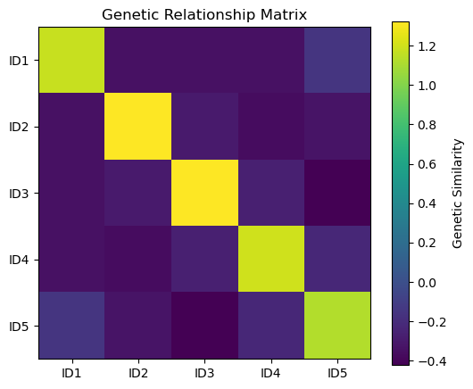
3.4 Simple Python Example: Simulating a GRM
import numpy as npimport pandas as pdnp.random.seed(42)# Simulate genotype matrix# rows = individuals# columns = SNPsn_individuals =5n_snps =100genotypes = np.random.randint(0, 3, size=(n_individuals, n_snps))# Allele frequenciesp = genotypes.mean(axis=0) /2# Standardize genotypesZ = (genotypes -2* p) / np.sqrt(2* p * (1- p) +1e-8)# Compute GRMGRM = (Z @ Z.T) / n_snpsgrm_df = pd.DataFrame( GRM, columns=[f"ID{i+1}"for i inrange(n_individuals)], index=[f"ID{i+1}"for i inrange(n_individuals)])grm_df.round(3)
ID1
ID2
ID3
ID4
ID5
ID1
1.181
-0.343
-0.344
-0.345
-0.149
ID2
-0.343
1.322
-0.293
-0.359
-0.326
ID3
-0.344
-0.293
1.324
-0.266
-0.420
ID4
-0.345
-0.359
-0.266
1.196
-0.226
ID5
-0.149
-0.326
-0.420
-0.226
1.121
3.5 Visualizing the GRM
import matplotlib.pyplot as pltplt.figure(figsize=(6,5))plt.imshow(GRM)plt.colorbar(label="Genetic Similarity")plt.title("Genetic Relationship Matrix")plt.xticks(range(n_individuals), grm_df.columns)plt.yticks(range(n_individuals), grm_df.index)plt.show()
3.6 Summary
The Genetic Relationship Matrix (GRM) measures genome-wide genetic similarity between individuals and forms the foundation of many modern statistical genetics methods.
Population stratification refers to ancestry differences within datasets that can create false associations in GWAS.
These concepts are deeply connected because ancestry influences genome-wide genetic similarity.
Modern GWAS pipelines routinely combine:
PCA correction,
GRM-based mixed models,
ancestry filtering,
genomic inflation diagnostics
to produce robust and reliable association results.
3.7 References
Yang J et al. (2011). GCTA: A Tool for Genome-wide Complex Trait Analysis.
Price AL et al. (2006). Principal Components Analysis Corrects for Stratification in GWAS.
Patterson N et al. (2006). Population Structure and Eigenanalysis.
Lee SH et al. (2012). Estimation of SNP Heritability.