Covariance and correlation are two of the most fundamental concepts in statistics, data science, machine learning, finance, genomics, and many other quantitative fields.
Both concepts attempt to answer an important question:
How do two variables change together?
For example:
Do height and weight increase together?
Do gene expression levels move together?
Does temperature increase electricity usage?
Do stock prices move in the same direction?
Covariance and correlation help quantify these relationships mathematically.
Although they are closely related, they are not identical.
This tutorial explains:
what covariance is,
what correlation is,
how they differ,
how they are computed,
and how to interpret them correctly.
What is Variability?
Before discussing covariance, it is important to understand variance.
Variance measures:
how much a variable varies around its mean.
For a variable ( X ):
$ (X) = _{i=1}^{n} (X_i - {X})^2 $
Variance tells us:
whether observations are tightly clustered,
or widely spread out.
Covariance extends this idea to two variables simultaneously.
What is Covariance?
Covariance measures:
how two variables vary together.
It tells us whether:
variables increase together,
decrease together,
or move in opposite directions.
Intuition Behind Covariance
Consider the term:
$ (X_i - {X})(Y_i - {Y}) $
There are several possibilities.
Case 1: Both Variables Increase Together
If:
( X_i > {X} )
and ( Y_i > {Y} )
then:
[ (+)(+) = + ]
This contributes positively.
Similarly:
both below their means also produce positive values.
Thus:
positive covariance indicates variables move together.
Case 2: Variables Move Oppositely
If:
( X_i > {X} )
but ( Y_i < {Y} )
then:
$ (+)(-) = - $
This contributes negatively.
Negative covariance indicates opposite movement.
Interpretation of Covariance
Positive
Variables increase together
Negative
One increases while the other decreases
Near zero
Weak or no linear relationship
Important Limitation of Covariance
Covariance depends on scale.
For example:
covariance between income and spending may be extremely large,
covariance between height and weight may be smaller.
This makes covariance difficult to interpret directly.
To solve this problem, we use correlation.
What is Correlation?
Correlation is a standardized version of covariance.
It measures:
both the strength and direction of a linear relationship.
Unlike covariance, correlation is scale-independent.
Why Standardization Matters
By dividing covariance by standard deviations:
units cancel out,
the measure becomes dimensionless,
interpretation becomes easier.
Range of Correlation
Correlation always lies between:
$ -1 r $
Interpretation of Correlation
+1
perfect positive relationship
+0.8
strong positive relationship
+0.5
moderate positive relationship
0
no linear relationship
-0.5
moderate negative relationship
-1
perfect negative relationship
Positive Correlation
Positive correlation means:
as one variable increases,
the other also tends to increase.
Examples:
height and weight,
study time and exam score,
income and expenditure.
Negative Correlation
Negative correlation means:
as one variable increases,
the other tends to decrease.
Examples:
exercise and body fat,
speed and travel time,
stress and sleep quality.
Zero Correlation
Zero correlation indicates:
no linear relationship.
However, this does NOT always mean the variables are unrelated.
They may still have:
nonlinear relationships,
curved relationships,
threshold effects.
Correlation Does Not Imply Causation
One of the most important statistical principles is:
correlation does not imply causation.
If two variables are correlated, it does not necessarily mean:
There may be:
confounding variables,
indirect relationships,
coincidence,
shared causes.
Example of Confounding
Suppose:
ice cream sales increase,
drowning incidents also increase.
This does not mean:
ice cream causes drowning.
The hidden factor is:
Covariance Matrix
In multivariate statistics, covariance is often represented as a matrix.
For variables ( X_1, X_2, X_3 ):
$ =
\[\begin{bmatrix}
\text{Var}(X_1) & \text{Cov}(X_1,X_2) & \text{Cov}(X_1,X_3) \\
\text{Cov}(X_2,X_1) & \text{Var}(X_2) & \text{Cov}(X_2,X_3) \\
\text{Cov}(X_3,X_1) & \text{Cov}(X_3,X_2) & \text{Var}(X_3)
\end{bmatrix}\]
$
Covariance matrices are fundamental in:
PCA,
multivariate Gaussian models,
machine learning,
genomics,
finance.
Correlation Matrix
Similarly, correlation matrices contain pairwise correlations.
All diagonal values equal 1 because:
$ (X,X) = 1 $
Covariance vs Correlation
Measures joint variability
Yes
Yes
Indicates direction
Yes
Yes
Standardized
No
Yes
Scale dependent
Yes
No
Range fixed
No
Yes (-1 to 1)
Easy interpretation
Difficult
Easier
Covariance and Correlation in Genetics
These concepts are extremely important in genetics.
Examples include:
genetic covariance between traits,
linkage disequilibrium,
genetic correlation,
GRM construction,
polygenic score analysis.
For example:
schizophrenia and bipolar disorder show positive genetic correlation.
Covariance in PCA
Principal Component Analysis (PCA) operates on the covariance matrix.
PCA identifies directions of maximum variance.
This is widely used in:
GWAS population structure analysis,
dimensionality reduction,
transcriptomics.
# Python Example: Covariance and Correlation import numpy as npimport pandas as pd42 )# Simulated data = np.random.normal(10 , 2 , 100 )= x * 0.8 + np.random.normal(0 , 1 , 100 )= pd.DataFrame({"X" : x,"Y" : y
0
10.993428
7.379372
1
9.723471
7.358132
2
11.295377
8.693587
3
13.046060
9.634571
4
9.531693
7.464069
# Computing Covariance = df.cov()print (covariance)# Computing Correlation = df.corr()print (correlation)
          X         Y
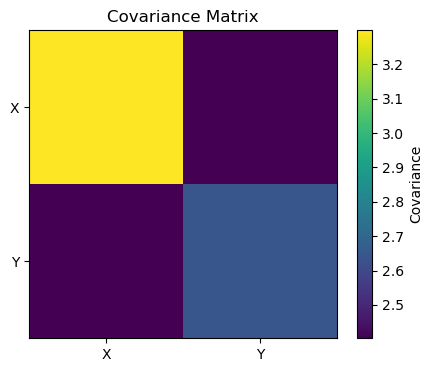
X  3.299080  2.402955
Y  2.402955  2.642802
          X         Y
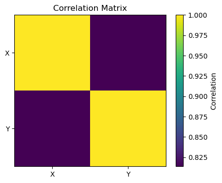
X  1.000000  0.813799
Y  0.813799  1.000000
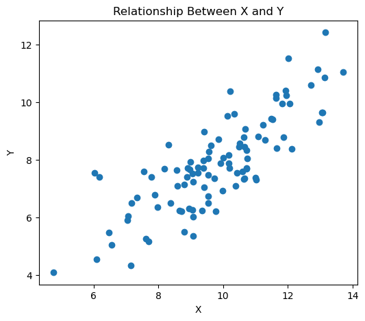
# Visualizing the Relationship import matplotlib.pyplot as plt= (6 ,5 ))"X" ], df["Y" ])"X" )"Y" )"Relationship Between X and Y" )
# Visualizing Covariance Matrix = (5 ,4 ))= "Covariance" )0 ,1 ], ["X" ,"Y" ])0 ,1 ], ["X" ,"Y" ])"Covariance Matrix" )
# Visualizing Correlation Matrix = (5 ,4 ))= "Correlation" )0 ,1 ], ["X" ,"Y" ])0 ,1 ], ["X" ,"Y" ])"Correlation Matrix" )
Why Covariance Matrices Are So Common in Statistical Genetics
Covariance matrices appear everywhere in statistical genetics because genetics itself is fundamentally about shared variation and dependence.
Individuals in genetic datasets are not completely independent. They may:
share ancestry,
share inherited genomic segments,
belong to the same family,
share environmental exposures,
or have correlated biological pathways.
A covariance matrix provides a mathematical way to describe these relationships.
In statistical genetics, many methods are essentially trying to answer questions like:
How genetically similar are two individuals?
How much phenotype similarity is explained by genotype similarity?
Which traits share genetic architecture?
Which variants move together because of linkage disequilibrium?
How much of the variance in a trait is explained by genetics?
All of these involve covariance structures.
Variance vs Covariance
Variance measures variability within one variable:
[ (X) ]
Covariance measures joint variability between two variables:
[ (X,Y) ]
A covariance matrix extends this idea to many variables simultaneously.
For variables ( X_1, X_2, …, X_n ):
$ =
\[\begin{bmatrix}
\text{Var}(X_1) & \text{Cov}(X_1,X_2) & \cdots \\
\text{Cov}(X_2,X_1) & \text{Var}(X_2) & \cdots \\
\vdots & \vdots & \ddots
\end{bmatrix}\]
$
This matrix summarizes the dependence structure of the system.
1. Genetic Relationship Matrix (GRM)
One of the most important covariance matrices in genetics is the Genetic Relationship Matrix (GRM).
The GRM measures genome-wide genetic similarity between individuals.
$ G = ZZ^T $
where:
( Z ) = standardized genotype matrix,
( M ) = number of SNPs.
The GRM is essentially a covariance matrix between individuals based on genotype data.
Interpretation:
large values → genetically similar individuals,
small values → unrelated individuals.
Why the GRM Matters
The GRM allows mixed models to account for:
family structure,
cryptic relatedness,
polygenic background,
ancestry effects.
This is critical in GWAS.
2. Covariance Structure in Linear Mixed Models
Modern GWAS often use linear mixed models:
$ y = X+ g + $
with:
$ g N(0, G_g^2) $
This means:
genetic effects are assumed to follow a multivariate normal distribution,
covariance between individuals is determined by the GRM.
The covariance matrix defines how phenotype correlations arise from genotype similarity.
3. SNP Heritability Estimation
Methods like GCTA-GREML estimate SNP heritability using covariance structures.
Core idea:
If genetically similar individuals also have similar phenotypes, then genetics explains part of the trait variance.
This is fundamentally a covariance argument.
The model compares:
covariance in genotype space, with
covariance in phenotype space.
4. Linkage Disequilibrium (LD)
Linkage disequilibrium measures correlation between nearby SNPs.
LD matrices are covariance/correlation matrices between variants.
Example:
[ R = (SNP_i, SNP_j) ]
LD matrices are essential in:
fine mapping,
PRS methods,
LD score regression,
Bayesian GWAS methods,
SBayesR,
SuSiE,
coloc.
5. Principal Component Analysis (PCA)
Population stratification correction often uses PCA.
PCA is performed on covariance-like structures derived from genotype matrices.
The eigenvectors of these covariance matrices reveal ancestry axes.
Thus, covariance matrices help uncover:
population structure,
ancestry clusters,
hidden stratification.
6. Genetic Correlation Between Traits
Methods like LDSC estimate genetic correlation between traits.
Example:
schizophrenia and bipolar disorder,
BMI and type 2 diabetes.
These methods estimate covariance of SNP effect sizes across traits.
Positive covariance suggests shared biology.
7. Multivariate Genetics
Multivariate genetic models directly model covariance between traits.
For example:
$ _G =
\[\begin{bmatrix}
\text{Var}(Trait_1) & \text{Cov}(Trait_1,Trait_2) \\
\text{Cov}(Trait_2,Trait_1) & \text{Var}(Trait_2)
\end{bmatrix}\]
$
This allows researchers to estimate:
shared heritability,
pleiotropy,
common pathways.
8. Bayesian Statistical Genetics
Bayesian methods heavily rely on covariance structures.
Examples include:
Gaussian processes,
multivariate priors,
LD-aware models,
random effect models.
Covariance matrices define prior dependence between variables.
9. Omics Data Are High-Dimensional
Modern genomics involves:
transcriptomics,
methylation,
proteomics,
metabolomics.
These datasets contain thousands of correlated variables.
Covariance matrices summarize their dependence structure efficiently.
10. Biological Systems Are Networked
Genes do not function independently.
They operate in:
pathways,
regulatory networks,
co-expression modules.
Covariance matrices naturally describe coordinated biological behavior.
Why Covariance Is More Important Than Mean Effects
In many classical statistical problems, the main focus is estimating mean effects.
In statistical genetics, much of the focus shifts toward:
covariance,
variance partitioning,
dependence structures,
random effects.
This is because most complex traits are highly polygenic.
Thousands of variants contribute tiny correlated effects.
A Deep Conceptual Point
Many statistical genetics methods are based on this idea:
Similar genomes should produce similar phenotypes.
This statement is fundamentally about covariance.
If:
genotype covariance predicts phenotype covariance,
then genetic effects exist.
This simple idea underlies:
heritability estimation,
mixed models,
genomic prediction,
polygenic risk scores.
Covariance Matrices in Practice
Covariance matrices appear in:
GCTA
GRM
PCA
Covariance matrix
LDSC
LD covariance
SBayesR
LD matrix
Mixed models
Random effect covariance
Genomic prediction
Genomic covariance
eQTL analysis
Expression covariance
TWAS
SNP-expression covariance
Covariance matrices are central in statistical genetics because genetics is fundamentally about shared variation and dependence.
They allow researchers to model:
relatedness,
linkage disequilibrium,
population structure,
polygenic effects,
shared heritability,
and biological networks.
Modern statistical genetics is therefore heavily built around covariance structures and multivariate modeling.
Summary
Covariance measures how two variables vary together, while correlation measures the strength and direction of their standardized linear relationship.
Covariance is scale-dependent and difficult to compare across datasets, whereas correlation is standardized between -1 and 1 and easier to interpret.
These concepts are foundational in:
statistics,
machine learning,
genomics,
finance,
signal processing,
and multivariate analysis.
Understanding covariance and correlation is essential for interpreting relationships between variables and for building more advanced statistical models.
References
James G et al. (2021). An Introduction to Statistical Learning.
Hastie T, Tibshirani R, Friedman J. The Elements of Statistical Learning.
Bishop CM. Pattern Recognition and Machine Learning.
Johnson RA, Wichern DW. Applied Multivariate Statistical Analysis.
Pearson K. Mathematical Contributions to the Theory of Evolution.