Multivariate Concepts in Statistical Genetics: From LD Score Regression to Genomic SEM
A Step-by-Step Practical Tutorial
Statistical Genetics
GWAS
Genomic SEM
Multivariate Analysis
How LD Score Regression extends from single-trait heritability to cross-trait genetic covariance, and how Genomic SEM fits structural models – common factors, regressions, GWAS-by-subtraction – to that covariance structure.
Author
Nivedita Bhadra
Published
July 28, 2026
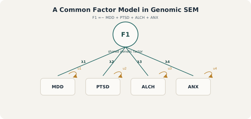
The model this tutorial builds up to fitting: a single shared genetic factor F1, estimated not from individual-level data but from a genetic covariance matrix built out of GWAS summary statistics alone.
Genomic SEMLDSCStructural Equation ModelingR
1 Multivariate Concepts in Statistical Genetics
In many areas of statistical genetics, we are not only interested in whether a single trait is heritable. We are also interested in whether multiple traits share part of their genetic architecture.
For example, psychiatric traits such as major depression, anxiety, post-traumatic stress disorder, alcohol use disorder, bipolar disorder, and schizophrenia are not genetically isolated. They often show genetic overlap. This means that some genetic variants may influence more than one phenotype.
This tutorial introduces the main multivariate concepts needed to understand Genomic SEM. We will move step by step from basic ideas such as polygenicity and LD Score Regression to genetic covariance, genetic correlation, genome-wide structural models, and multivariate GWAS.
1.0.1 1. Why Do We Need Multivariate Genetic Models?
Complex traits are usually highly polygenic. This means that they are influenced by thousands of genetic variants, each with a very small effect.
A simple single-gene model is usually not appropriate for complex psychiatric or behavioral traits. Instead, risk emerges from the combined effect of many variants.
This creates two important problems:
We need methods that can summarize genome-wide genetic signal.
We need methods that can estimate how much genetic signal is shared across traits.
This is where LD Score Regression and Genomic SEM become useful.
1.0.2 2. From Genetic Overlap to Genetic Architecture
Genetic overlap means that the same genetic variants contribute to variation in more than one phenotype.
However, genetic overlap can appear in different forms.
Two traits may share:
A broad common genetic factor Several smaller domain-specific factors A mixture of shared and trait-specific genetic effects SNPs that influence one trait much more than another
Genomic SEM allows us to model these possibilities explicitly.
For example, if four psychiatric traits are genetically correlated, we can test whether this correlation is well explained by one common factor.
A simplified model could be:
$ F_1 MDD, PTSD, ANX, ALCH $
where \((F_1)\) is a shared genetic liability factor.
1.0.3 3. Why Traits Do Not Need to Come From the Same Sample
One powerful feature of LD Score Regression and Genomic SEM is that traits do not need to be measured in the same individuals.
For example, we may have:
A GWAS of major depression from one cohort A GWAS of anxiety from another cohort A GWAS of PTSD from another cohort A GWAS of alcohol use disorder from another cohort
These GWAS may come from different studies, different consortia, and different individuals.
The connection between them is the genome.
Because each GWAS reports SNP-level effects across the genome, we can compare the pattern of SNP effects across traits. If SNPs that increase one trait also tend to increase another trait, this creates evidence of shared genetic architecture.
This is why summary statistics are so useful. We do not always need access to individual-level data to study genetic overlap.
1.0.4 2. Polygenicity and Linkage Disequilibrium
Suppose a phenotype is influenced by a few true causal variants. In GWAS, we do not observe only those causal variants. We also observe many nearby SNPs that are correlated with them.
This correlation among SNPs is called linkage disequilibrium, or LD.
A SNP with high LD is correlated with many nearby SNPs. Therefore, high-LD SNPs are more likely to tag causal variants. This means they are more likely to show association signal even if they are not causal themselves.
1.0.4.1 2.1 LD Score
The LD score of SNP (j) is defined as:
$ _j = i r{ij}^2 $
where:
\(\ell_j\) is the LD score of SNP (j)
\(r_{ij}^2\) is the squared correlation between SNP (i) and SNP (j)
A high LD score means that the SNP is correlated with many other SNPs.
1.0.5 4. The Intuition Behind LD Score Regression
LD Score Regression works because highly polygenic traits create a predictable relationship between LD and GWAS signal.
Imagine there are true causal variants in the genome.
A SNP does not need to be causal to show association. If it is correlated with a causal variant through LD, it can still pick up association signal.
This means:
High-LD SNPs are correlated with many nearby SNPs. Therefore, they have more chances to tag causal variants. Low-LD SNPs are correlated with fewer nearby SNPs. Therefore, they usually only show strong signal if they are causal or very close to causal variants.
For a highly polygenic trait, many causal variants are spread across the genome. As a result, SNPs with higher LD scores tend to have larger GWAS chi-square statistics on average.
This is the core logic of LD Score Regression.
1.0.6 5. Why the LDSC Intercept Matters
In GWAS, test statistics can be inflated for several reasons.
Some inflation reflects true polygenic signal. This is expected when many SNPs contribute to the trait.
However, some inflation can come from confounding, such as:
Population stratification Cryptic relatedness Sample overlap Technical artifacts
LD Score Regression separates these components.
The slope of the regression captures polygenic signal.
The intercept captures inflation that is not explained by LD score.
This is why LD Score Regression is useful: it helps distinguish true polygenic signal from confounding.
1.0.7 3. SNP Heritability Using LD Score Regression
LD Score Regression is based on a simple idea:
If a trait is highly polygenic, SNPs with higher LD scores should, on average, have larger GWAS test statistics.
In other words, we regress the GWAS chi-square statistics on LD scores.
The expected chi-square statistic for SNP (j) can be written as:
$ E[_j^2 | _j] = _j + Na + 1 $
where:
\(N\) is the GWAS sample size
\(h^2\) is SNP heritability
\(M\) is the number of SNPs
\(\ell_j\) is the LD score
\(a\) captures confounding such as population stratification
the intercept captures inflation not due to polygenic signal
The slope of this regression is used to estimate SNP heritability.
1.0.7.1 3.1 Why Sample Size Matters
Imagine two traits have the same GWAS p-values, but different sample sizes:
Trait 1: \(N = 50,000\)
Trait 2: \(N = 100,000\)
If the association statistics are similar, the trait with the smaller sample size may imply stronger per-sample genetic signal. This is why LD Score Regression accounts for sample size when estimating heritability.
1.0.8 4. Genetic Covariance and Genetic Correlation
LD Score Regression can also be extended to two traits.
Instead of regressing one trait’s chi-square statistics on LD scores, we examine the product of GWAS (Z)-statistics across two traits.
For traits (Y_1) and (Y_2), we use:
$ Z_{1j}Z_{2j} $
If SNPs with high LD scores tend to have similar effects across both traits, this suggests genetic overlap.
1.0.8.1 4.1 Genetic Covariance
Genetic covariance measures the extent to which two traits share genetic influences.
The cross-trait LD Score Regression equation is:
$ E[z_{1j}z_{2j}|_j] = j + + {Ns} $
Conceptually:
The slope estimates genetic covariance.
The intercept captures sample overlap and confounding.
Traits do not need to be measured in the same individuals.
This is very useful because many GWAS summary statistics are publicly available and come from independent cohorts.
1.0.8.2 4.2 Genetic Correlation
Genetic correlation is the standardized form of genetic covariance:
$ r_g = {} $
A genetic correlation close to 1 means two traits share much of their genetic architecture.
A genetic correlation close to 0 means little shared genetic influence.
A negative genetic correlation means genetic variants that increase one trait tend to decrease the other.
1.0.9 8. Why Shared Genetic Architecture Requires New Models
1.0.10 5. From LD Score Regression to Genomic SEM
Genomic SEM stands for Genomic Structural Equation Modeling.
It provides a flexible framework for fitting structural equation models to genetic covariance matrices estimated from GWAS summary statistics.
The main advantage is that we can model genetic relationships among traits even when those traits were measured in different samples.
The downloaded binary packages are in
    /var/folders/3f/6pzn2nyn32d7wthyxkzsqyxcdrtvym/T//RtmpPbLU4V/downloaded_packages
──R CMD build─────────────────────────────────────────────────────────────────✔checking for file ‘/private/var/folders/3f/6pzn2nyn32d7wthyxkzsqyxcdrtvym/T/RtmpPbLU4V/remotes2dbf3fb76124/GenomicSEM-GenomicSEM-0a63ac0/DESCRIPTION’─preparing ‘GenomicSEM’:✔checking DESCRIPTION meta-information─excluding invalid files
Subdirectory 'man' contains invalid file names:
‘decisiontree.png’
─checking for LF line-endings in source and make files and shell scripts─checking for empty or unneeded directories
Omitted ‘LazyData’ from DESCRIPTION
─building ‘GenomicSEM_0.0.5.tar.gz’
Warning: invalid uid value replaced by that for user 'nobody'
Warning: invalid gid value replaced by that for user 'nobody'
library(GenomicSEM)
1.0.14 8. Step 1: Munge Summary Statistics
Munging is the process of cleaning and harmonizing GWAS summary statistics.
It usually includes:
Aligning alleles
Filtering to HapMap3 SNPs
Checking SNP IDs
Formatting effect sizes
Formatting standard errors
Preparing files for LD Score Regression
In this practical, the workshop uses four traits:
ALCH: Alcohol use disorder
PTSD: Post-traumatic stress disorder
MDD: Major depressive disorder
ANX: Anxiety disorder
# Example file namesfiles <-c("ALCH_withrsID.txt","SORTED_PTSD_EA9_ALL_study_specific_PCs1.txt","MDD_withNeff.txt","ANX_withNeff.txt")# HapMap3 SNP reference filehm3 <-"eur_w_ld_chr/w_hm3.snplist"# Trait namestrait.names <-c("ALCH", "PTSD", "MDD", "ANX")# Effective sample sizeN <-c(NA, 5831.346, NA, NA)# Run munge# This is commented out because the workshop already provides prepared files.# munge(files = files, hm3 = hm3, trait.names = trait.names, N = N)
1.0.15 9. Step 2: Run Multivariable LD Score Regression
After munging, we run LD Score Regression.
This estimates:
SNP heritability for each trait
Genetic covariance between traits
Genetic correlation between traits
Sampling covariance matrix
The output is later used by Genomic SEM.
# Munged summary statisticstraits <-c("ALCH.sumstats.gz","PTSD.sumstats.gz","MDD.sumstats.gz","ANX.sumstats.gz")# Sample prevalencesample.prev <-c(.5, .5, .5, .5)# Population prevalencepopulation.prev <-c(.159, .3, .15, .20)# LD score foldersld <-"eur_w_ld_chr/"wld <-"eur_w_ld_chr/"# Trait namestrait.names <-c("ALCH", "PTSD", "MDD", "ANX")# Run LDSC# This is commented out because the workshop provides LDSC_INT.RData.# LDSC_INT <- ldsc(# traits = traits,# sample.prev = sample.prev,# population.prev = population.prev,# ld = ld,# wld = wld,# trait.names = trait.names# )# Save LDSC output# save(LDSC_INT, file = "LDSC_INT.RData")
1.0.16 10. Step 3: Load the LDSC Output
The workshop practical already provides the LDSC object.
This object contains the genetic covariance matrix and sampling covariance matrix.
Latent factors do not have a natural scale. Therefore, we must identify the scale of the factor.
There are two common approaches.
Option 1: Unit Variance Identification
In this approach, the variance of the latent factor is fixed to 1.
Example:
Model <- ” F1 =~ NAMDD + PTSD + ALCH + ANX F1 1F1 ”
This means the factor has a standardized variance.
In Genomic SEM, this is often equivalent to using:
std.lv = TRUE Option 2: Unit Loading Identification
In this approach, one factor loading is fixed to 1.
Example:
Model <- ” F1 =~ 1*MDD + PTSD + ALCH + ANX ”
Here, the scale of the factor is defined by MDD.
Both approaches are valid, but they lead to different parameter scaling. The interpretation of the model should always consider how the factor was identified.
1.0.20 13. Lavaan Model Syntax Used in Genomic SEM
Genomic SEM uses lavaan-style model syntax.
Here are the most important operators:
Syntax
Meaning
A ~ B
A is regressed on B
A ~~ A
Variance of A
A ~~ B
Covariance between A and B
F1 =~ A + B + C
Latent factor F1 loads on A, B, and C
A ~~ 1*B
Fix covariance between A and B to 1
A ~~ a*B
Label covariance as parameter a
This syntax allows us to specify many different genetic models.
1.0.21 14. Common Factor Model
A common factor model assumes that several observed traits share one underlying latent genetic factor.
For example:
$ F1 MDD, PTSD, ALCH, ANX $
Here, F1 represents a shared internalizing genetic factor.
# Define covariance structurecovstruc <- LDSC_INT# Common factor modelINT.model <-"F1 =~ MDD + PTSD + ALCH + ANX"# Use unit variance identificationstd.lv <-TRUE# Run modelIntResults <-usermodel(covstruc = covstruc,model = INT.model,std.lv = std.lv)
Genomic SEM is not limited to factor models. It can also estimate genetic regression models.
For example, suppose we want to know whether the genetic component of educational attainment is associated with schizophrenia and bipolar disorder.
A simplified model could be:
[ EA_g = b_1SCZ_g + b_2BIP_g + u]
This means that the genetic component of educational attainment is regressed on the genetic components of schizophrenia and bipolar disorder.
In lavaan-style syntax, this could be written as:
model <- ” EA ~ SCZ + BIP SCZ BIP ”
This allows us to ask whether one trait explains unique genetic variation in another trait after accounting for additional genetically correlated traits.
1.0.23 16. GWAS-by-Subtraction
GWAS-by-subtraction is one of the important applications of Genomic SEM.
The idea is to separate shared and residual genetic components.
For example, educational attainment and cognitive performance are genetically correlated. But educational attainment is influenced by both cognitive and non-cognitive factors.
A Genomic SEM model can estimate:
A cognitive genetic factor shared with cognitive performance A non-cognitive genetic component of educational attainment
Conceptually:
$ EA = Cognitive + NonCognitive $
This allows researchers to perform GWAS on the residual non-cognitive component.
In simple terms, GWAS-by-subtraction asks:
What genetic signal remains in one trait after removing the genetic signal shared with another trait?
This is useful when we want to isolate more specific genetic pathways.
1.0.24 15. View Model Results
The results table contains:
Parameter estimates
Standard errors
Standardized estimates
p-values
The factor loadings tell us how strongly each trait relates to the latent genetic factor.
IntResults$results
A data.frame: 9 × 9
lhs
op
rhs
Unstand_Est
Unstand_SE
STD_Genotype
STD_Genotype_SE
STD_All
p_value
<chr>
<chr>
<chr>
<dbl>
<chr>
<dbl>
<chr>
<dbl>
<dbl>
5
F1
=~
MDD
0.283806747
0.021002745436444
0.97326125
0.0720249151052966
0.97326125
1.313540e-41
6
F1
=~
PTSD
0.221278068
0.0402049336545347
0.45226835
0.0821745168725034
0.45226834
3.717880e-08
3
F1
=~
ALCH
0.205225639
0.024321802328951
0.54969157
0.0651453167330757
0.54969157
3.230100e-17
4
F1
=~
ANX
0.445784749
0.032456114148652
0.92294074
0.0671962594562505
0.92294072
6.265550e-43
1
ALCH
~~
ALCH
0.097270350
0.025899146459423
0.69783919
0.185806270387686
0.69783918
1.728330e-04
9
PTSD
~~
PTSD
0.190414108
0.106977265864464
0.79545336
0.446896663140437
0.79545335
7.508426e-02
8
MDD
~~
MDD
0.004486541
0.0109566843706871
0.05276254
0.12885240976165
0.05276254
6.821876e-01
2
ANX
~~
ANX
0.034569558
0.0301103378331493
0.14818043
0.129066285535458
0.14818043
2.509289e-01
7
F1
~~
F1
1.000000000
1.00000000
1.00000000
NA
1.0.25 16. View Model Fit
Model fit tells us whether the proposed model explains the observed genetic covariance matrix well.
Important fit statistics include:
Chi-square: lower is better
AIC: useful for comparing models
CFI: higher is better
SRMR: lower is better
As a rough guide:
CFI > 0.90 suggests acceptable fit
CFI > 0.95 suggests good fit
SRMR < 0.10 suggests acceptable fit
SRMR < 0.05 suggests good fit
IntResults$modelfit
A data.frame: 1 × 6
chisq
df
p_chisq
AIC
CFI
SRMR
<dbl>
<dbl>
<dbl>
<dbl>
<dbl>
<dbl>
df
1.283452
2
0.526383
17.28345
1
0.03621695
1.0.26 17. Interpreting the Common Factor Model
A strong loading of MDD on F1 means that major depression strongly reflects the shared genetic factor.
A weaker loading of ALCH on F1 means that alcohol use disorder may share some genetic risk with the factor, but also has more trait-specific genetic influences.
The residual variance of each trait represents genetic variation not explained by the common factor.
1.0.27 18. Alternative Model: Correlated Traits Model
Instead of forcing all traits to load on a common factor, we could estimate pairwise genetic covariances directly.
This is useful when we do not want to assume a latent factor.
[1] "Running primary model"
[1] "Calculating Standardized Results"
[1] "Calculating SRMR"
elapsed
  0.104
[1] "Model fit statistics are all printed as NA as you have specified a fully saturated model (i.e., df = 0)"
A data.frame: 10 × 9
lhs
op
rhs
Unstand_Est
Unstand_SE
STD_Genotype
STD_Genotype_SE
STD_All
p_value
<chr>
<chr>
<chr>
<dbl>
<dbl>
<dbl>
<dbl>
<dbl>
<dbl>
7
MDD
~~
PTSD
0.05799439
0.011560951
0.4064906
0.08103228
0.4064906
5.264780e-07
4
MDD
~~
ALCH
0.05943021
0.006076568
0.5458853
0.05581520
0.5458853
1.369039e-22
5
MDD
~~
ANX
0.12667327
0.007147882
0.8993739
0.05074961
0.8993739
2.847008e-70
8
PTSD
~~
ALCH
0.05977947
0.041025806
0.3272633
0.22459619
0.3272633
1.450836e-01
9
PTSD
~~
ANX
0.11428679
0.028723611
0.4836180
0.12154733
0.4836180
6.925092e-05
2
ALCH
~~
ANX
0.08500236
0.016208124
0.4713755
0.08988118
0.4713755
1.567668e-07
1
ALCH
~~
ALCH
0.13938790
0.024579672
1.0000000
0.17634007
1.0000000
1.420817e-08
10
PTSD
~~
PTSD
0.23937808
0.106582777
1.0000000
0.44524869
1.0000000
2.470812e-02
6
MDD
~~
MDD
0.08503281
0.003491874
1.0000000
0.04106502
1.0000000
5.572026e-131
3
ANX
~~
ANX
0.23329361
0.016862213
1.0000000
0.07227893
1.0000000
1.561049e-43
A data.frame: 1 × 6
chisq
df
p_chisq
AIC
CFI
SRMR
<lgl>
<dbl>
<lgl>
<lgl>
<lgl>
<lgl>
df
NA
0
NA
NA
NA
NA
1.0.28 19. Alternative Model: Regression Model
Genomic SEM can also fit genetic regression models.
For example, we can ask whether the genetic component of anxiety predicts the genetic component of depression.
[1] "Running primary model"
[1] "Calculating Standardized Results"
[1] "Calculating SRMR"
elapsed
  0.115
[1] "Model fit statistics are all printed as NA as you have specified a fully saturated model (i.e., df = 0)"
A data.frame: 10 × 9
lhs
op
rhs
Unstand_Est
Unstand_SE
STD_Genotype
STD_Genotype_SE
STD_All
p_value
<chr>
<chr>
<chr>
<dbl>
<dbl>
<dbl>
<dbl>
<dbl>
<dbl>
7
MDD
~
ANX
0.51330125
0.068314744
0.85021835
0.11315470
0.85021835
5.744864e-14
8
MDD
~
PTSD
-0.03483028
0.094099604
-0.05843942
0.15788349
-0.05843942
7.112762e-01
6
MDD
~
ALCH
0.12827888
0.075097732
0.16423830
0.09614929
0.16423830
8.760680e-02
4
ANX
~~
PTSD
0.11428679
0.028723611
0.48361796
0.12154733
0.48361796
6.925093e-05
2
ANX
~~
ALCH
0.08500236
0.016208124
0.47137552
0.08988118
0.47137551
1.567668e-07
9
PTSD
~~
ALCH
0.05977947
0.041025806
0.32726331
0.22459619
0.32726331
1.450836e-01
1
ALCH
~~
ALCH
0.13938790
0.024579672
1.00000001
0.17634007
1.00000001
1.420816e-08
10
PTSD
~~
PTSD
0.23937808
0.106582777
0.99999999
0.44524869
0.99999999
2.470812e-02
5
MDD
~~
MDD
0.01440758
0.005525258
0.16943560
0.06497795
0.16943560
9.118313e-03
3
ANX
~~
ANX
0.23329361
0.016862213
1.00000000
0.07227893
1.00000000
1.561050e-43
A data.frame: 1 × 6
chisq
df
p_chisq
AIC
CFI
SRMR
<lgl>
<dbl>
<lgl>
<lgl>
<lgl>
<lgl>
df
NA
0
NA
NA
NA
NA
1.0.29 20. Multivariate GWAS in Genomic SEM
So far, we estimated a genome-wide model using the genetic covariance matrix.
Now we move to multivariate GWAS.
The goal is to test SNP effects on a latent factor.
Instead of asking:
Is this SNP associated with MDD?
we ask:
Is this SNP associated with the shared genetic factor underlying MDD, PTSD, ALCH, and ANX?
This can increase power and improve interpretation when traits share genetic architecture.
1.0.30 21. Steps for Multivariate GWAS
Multivariate GWAS in Genomic SEM has four main steps:
Munge summary statistics
Run LD Score Regression
Prepare summary statistics using sumstats
Run multivariate GWAS using userGWAS
The first two steps are the same as before. If we already ran LDSC for the same traits, we do not need to repeat it.
1.0.31 22. Step 3 for Multivariate GWAS: Prepare SNP Summary Statistics
The sumstats() function prepares SNP-level summary statistics for userGWAS.
In the workshop practical, reduced chromosome 4 files are used for demonstration.
# Files must be in the same order as the LDSC traitsfiles <-c("ALCH4.txt", "PTSD4.txt", "MDD4.txt", "ANX4.txt")# Reference file for allele frequencyref <-"reference.1000G.ch4.txt"# Trait namestrait.names <-c("ALCH", "PTSD", "MDD", "ANX")# Whether SEs are on logistic scalese.logit <-c(FALSE, TRUE, TRUE, TRUE)# Whether linear probability model correction is neededlinprob <-c(TRUE, FALSE, FALSE, FALSE)# Sample size argumentN <-c(NA, NA, NA, NA)# Prepare summary statisticsINT_sumstats <-sumstats(files = files,ref = ref,trait.names = trait.names,se.logit = se.logit,linprob = linprob,N = N)
The preparation of 4 summary statistics for use in Genomic SEM began at: 2026-06-10 12:44:42.44117
Please note that the files should be in the same order that they were listed for the ldsc function
Reading in reference file
Applying MAF filer of 0.01 to the reference file.
All files loaded into R!
Preparing summary statistics for file: /Users/nbhadra/Documents/aSchork/ISG_2026/Scripts/script_day6/GenomicSEM_2026/ALCH4.txt
Interpreting the SNP column as the SNP column.
Interpreting the A1 column as the A1 column.
Interpreting the A2 column as the A2 column.
Interpreting the Z column as the effect column.
Interpreting the P column as the P column.
Interpreting the WEIGHT column as the N column.
0 rows were removed from the /Users/nbhadra/Documents/aSchork/ISG_2026/Scripts/script_day6/GenomicSEM_2026/ALCH4.txt summary statistics file due to entries that were duplicated for rsID. These are removed as they likely reflect multiallelic variants.
Merging file: /Users/nbhadra/Documents/aSchork/ISG_2026/Scripts/script_day6/GenomicSEM_2026/ALCH4.txt with the reference file: /Users/nbhadra/Documents/aSchork/ISG_2026/Scripts/script_day6/GenomicSEM_2026/reference.1000G.ch4.txt
1000 rows present in the full /Users/nbhadra/Documents/aSchork/ISG_2026/Scripts/script_day6/GenomicSEM_2026/ALCH4.txt summary statistics file.
0 rows were removed from the /Users/nbhadra/Documents/aSchork/ISG_2026/Scripts/script_day6/GenomicSEM_2026/ALCH4.txt summary statistics file as the rsIDs for these SNPs were not present in the reference file.
The effect column was determined NOT to be coded as an odds ratio (OR) for the /Users/nbhadra/Documents/aSchork/ISG_2026/Scripts/script_day6/GenomicSEM_2026/ALCH4.txt summary statistics file based on the median of the effect column being close to 0.
An transformation used to back out logistic betas for binary traits is being applied for: /Users/nbhadra/Documents/aSchork/ISG_2026/Scripts/script_day6/GenomicSEM_2026/ALCH4.txt
No INFO column, cannot filter on INFO, which may influence results
1000 SNPs are left in the summary statistics file /Users/nbhadra/Documents/aSchork/ISG_2026/Scripts/script_day6/GenomicSEM_2026/ALCH4.txt after QC and merging with the reference file.
Preparing summary statistics for file: /Users/nbhadra/Documents/aSchork/ISG_2026/Scripts/script_day6/GenomicSEM_2026/PTSD4.txt
Interpreting the MARKERNAME column as the SNP column.
Interpreting the ALLELE1 column as the A1 column.
Interpreting the ALLELE2 column as the A2 column.
Interpreting the EFFECT column as the effect column.
Interpreting the P.VALUE column as the P column.
Cannot find N column, try renaming it to N in the summary statistics file for:/Users/nbhadra/Documents/aSchork/ISG_2026/Scripts/script_day6/GenomicSEM_2026/PTSD4.txt
Interpreting the STDERR column as the SE column.
Interpreting the DIRECTION column as the DIRECTION column.
0 rows were removed from the /Users/nbhadra/Documents/aSchork/ISG_2026/Scripts/script_day6/GenomicSEM_2026/PTSD4.txt summary statistics file due to entries that were duplicated for rsID. These are removed as they likely reflect multiallelic variants.
Merging file: /Users/nbhadra/Documents/aSchork/ISG_2026/Scripts/script_day6/GenomicSEM_2026/PTSD4.txt with the reference file: /Users/nbhadra/Documents/aSchork/ISG_2026/Scripts/script_day6/GenomicSEM_2026/reference.1000G.ch4.txt
1000 rows present in the full /Users/nbhadra/Documents/aSchork/ISG_2026/Scripts/script_day6/GenomicSEM_2026/PTSD4.txt summary statistics file.
0 rows were removed from the /Users/nbhadra/Documents/aSchork/ISG_2026/Scripts/script_day6/GenomicSEM_2026/PTSD4.txt summary statistics file as the rsIDs for these SNPs were not present in the reference file.
The effect column was determined NOT to be coded as an odds ratio (OR) for the /Users/nbhadra/Documents/aSchork/ISG_2026/Scripts/script_day6/GenomicSEM_2026/PTSD4.txt summary statistics file based on the median of the effect column being close to 0.
No INFO column, cannot filter on INFO, which may influence results
Performing transformation under the assumption that the effect column is either an odds ratio or logistic beta (please see output above to determine whether it was interpreted as an odds ratio) and the SE column is a logistic SE (i.e., NOT the SE of the odds ratio) for:/Users/nbhadra/Documents/aSchork/ISG_2026/Scripts/script_day6/GenomicSEM_2026/PTSD4.txt
1000 SNPs are left in the summary statistics file /Users/nbhadra/Documents/aSchork/ISG_2026/Scripts/script_day6/GenomicSEM_2026/PTSD4.txt after QC and merging with the reference file.
Preparing summary statistics for file: /Users/nbhadra/Documents/aSchork/ISG_2026/Scripts/script_day6/GenomicSEM_2026/MDD4.txt
Found an NEFF column for sample size.

Please note that this is likely effective sample size and should only be used for liability h^2 conversion for binary traits and that it should reflect the sum of effective sample sizes across cohorts.

Be aware that some NEFF columns reflect half of the effective sample size; the function will automatically double the column names if recognized [check above in .log file to determine if this is the case].
If the Neff value is halved in the summary stats, but not recognized by the munge function, this should be manually doubled prior to running munge.
Interpreting the MARKERNAME column as the SNP column.
Interpreting the A1 column as the A1 column.
Interpreting the A2 column as the A2 column.
Interpreting the LOGOR column as the effect column.
Interpreting the P column as the P column.
Interpreting the NEFF column as the N column.
Interpreting the MAF column as the MAF column.
Interpreting the STDERRLOGOR column as the SE column.
0 rows were removed from the /Users/nbhadra/Documents/aSchork/ISG_2026/Scripts/script_day6/GenomicSEM_2026/MDD4.txt summary statistics file due to entries that were duplicated for rsID. These are removed as they likely reflect multiallelic variants.
Merging file: /Users/nbhadra/Documents/aSchork/ISG_2026/Scripts/script_day6/GenomicSEM_2026/MDD4.txt with the reference file: /Users/nbhadra/Documents/aSchork/ISG_2026/Scripts/script_day6/GenomicSEM_2026/reference.1000G.ch4.txt
1400 rows present in the full /Users/nbhadra/Documents/aSchork/ISG_2026/Scripts/script_day6/GenomicSEM_2026/MDD4.txt summary statistics file.
20 rows were removed from the /Users/nbhadra/Documents/aSchork/ISG_2026/Scripts/script_day6/GenomicSEM_2026/MDD4.txt summary statistics file as the rsIDs for these SNPs were not present in the reference file.
The effect column was determined NOT to be coded as an odds ratio (OR) for the /Users/nbhadra/Documents/aSchork/ISG_2026/Scripts/script_day6/GenomicSEM_2026/MDD4.txt summary statistics file based on the median of the effect column being close to 0.
5rows were removed from the/Users/nbhadra/Documents/aSchork/ISG_2026/Scripts/script_day6/GenomicSEM_2026/MDD4.txtsummary statistics file due to effect values estimated at exactly 0 as this causes problems for matrix inversion necessary for later Genomic SEM analyses.
No INFO column, cannot filter on INFO, which may influence results
Performing transformation under the assumption that the effect column is either an odds ratio or logistic beta (please see output above to determine whether it was interpreted as an odds ratio) and the SE column is a logistic SE (i.e., NOT the SE of the odds ratio) for:/Users/nbhadra/Documents/aSchork/ISG_2026/Scripts/script_day6/GenomicSEM_2026/MDD4.txt
1375 SNPs are left in the summary statistics file /Users/nbhadra/Documents/aSchork/ISG_2026/Scripts/script_day6/GenomicSEM_2026/MDD4.txt after QC and merging with the reference file.
Preparing summary statistics for file: /Users/nbhadra/Documents/aSchork/ISG_2026/Scripts/script_day6/GenomicSEM_2026/ANX4.txt
Found an NEFF column for sample size.

Please note that this is likely effective sample size and should only be used for liability h^2 conversion for binary traits and that it should reflect the sum of effective sample sizes across cohorts.

Be aware that some NEFF columns reflect half of the effective sample size; the function will automatically double the column names if recognized [check above in .log file to determine if this is the case].
If the Neff value is halved in the summary stats, but not recognized by the munge function, this should be manually doubled prior to running munge.
Interpreting the SNP column as the SNP column.
Interpreting the ALLELE1 column as the A1 column.
Interpreting the ALLELE2 column as the A2 column.
Interpreting the EFFECT column as the effect column.
Interpreting the P column as the P column.
Interpreting the NEFF column as the N column.
Interpreting the STDERR column as the SE column.
Interpreting the DIRECTION column as the DIRECTION column.
0 rows were removed from the /Users/nbhadra/Documents/aSchork/ISG_2026/Scripts/script_day6/GenomicSEM_2026/ANX4.txt summary statistics file due to entries that were duplicated for rsID. These are removed as they likely reflect multiallelic variants.
Merging file: /Users/nbhadra/Documents/aSchork/ISG_2026/Scripts/script_day6/GenomicSEM_2026/ANX4.txt with the reference file: /Users/nbhadra/Documents/aSchork/ISG_2026/Scripts/script_day6/GenomicSEM_2026/reference.1000G.ch4.txt
1000 rows present in the full /Users/nbhadra/Documents/aSchork/ISG_2026/Scripts/script_day6/GenomicSEM_2026/ANX4.txt summary statistics file.
0 rows were removed from the /Users/nbhadra/Documents/aSchork/ISG_2026/Scripts/script_day6/GenomicSEM_2026/ANX4.txt summary statistics file as the rsIDs for these SNPs were not present in the reference file.
The effect column was determined NOT to be coded as an odds ratio (OR) for the /Users/nbhadra/Documents/aSchork/ISG_2026/Scripts/script_day6/GenomicSEM_2026/ANX4.txt summary statistics file based on the median of the effect column being close to 0.
No INFO column, cannot filter on INFO, which may influence results
Performing transformation under the assumption that the effect column is either an odds ratio or logistic beta (please see output above to determine whether it was interpreted as an odds ratio) and the SE column is a logistic SE (i.e., NOT the SE of the odds ratio) for:/Users/nbhadra/Documents/aSchork/ISG_2026/Scripts/script_day6/GenomicSEM_2026/ANX4.txt
1000 SNPs are left in the summary statistics file /Users/nbhadra/Documents/aSchork/ISG_2026/Scripts/script_day6/GenomicSEM_2026/ANX4.txt after QC and merging with the reference file.
After merging across all summary statistics using listwise deletion, performing QC, and merging with the reference file, there are 1000 SNPs left in the final multivariate summary statistics file
Sumstats finished running at 2026-06-10 12:44:44.381982
Running sumstats for all files took 0 minutes and 1.94081211090088 seconds
Please check the log file ALCH_PTSD_MDD_ANX_sumstats.log to ensure that all columns were interpreted correctly and no warnings were issued for any of the summary statistics files.
1.0.32 23. Why linprob Is Needed
Sometimes binary traits are analyzed as continuous outcomes, or the summary statistics contain only Z-statistics.
In these cases, Genomic SEM needs additional information to reconstruct the appropriate beta and standard error.
In this practical, linprob = TRUE is used for ALCH.
1.0.33 24. Step 4: Run userGWAS
Now we run a multivariate GWAS.
The model is:
$ F1 =~ MDD + PTSD + ALCH + ANX $
and then:
$ F1 SNP $
This tests whether each SNP predicts the shared latent genetic factor.
# Covariance structure from LDSCcovstruc <- LDSC_INT# SNP-level summary statisticsSNPs <- INT_sumstats# Multivariate GWAS modelmodel <-"F1 =~ MDD + PTSD + ALCH + ANXF1 ~ SNP"# Save only the SNP effect on F1sub <-"F1~SNP"# Practical uses serial processingparallel <-FALSE# Calculate QSNPQ_SNP <-TRUE# Run multivariate GWASINT_GWAS <-userGWAS(covstruc = covstruc,SNPs = SNPs,model = model,sub = sub,parallel = parallel,Q_SNP = Q_SNP)
[1] "Please note that an update was made to userGWAS on Sept 1 2023  so that the default behavior is to fix the measurement model using the fix_measurement argument."
[1] "Starting GWAS Estimation"
Running Model: 1
Running Model: 1000
elapsed
 26.264
1.0.34 25. View the First Rows of the Multivariate GWAS Output
The output contains:
SNP effect on the factor
Standard error
p-value
QSNP statistic
QSNP p-value
Warnings and errors
INT_GWAS[[1]][1:5, ]
A data.frame: 5 × 24
SNP
CHR
BP
MAF
A1
A2
lhs
op
rhs
free
⋯
Pval_Estimate
chisq
chisq_df
chisq_pval
AIC
Q_SNP
Q_SNP_df
Q_SNP_pval
error
warning
<chr>
<int>
<int>
<dbl>
<chr>
<chr>
<chr>
<chr>
<chr>
<int>
⋯
<dbl>
<dbl>
<dbl>
<dbl>
<dbl>
<dbl>
<dbl>
<dbl>
<dbl>
<chr>
1
rs10030871
4
68786
0.0765408
T
C
F1
~
SNP
6
⋯
0.8257532
4.905573
8
0.7676193
18.90557
3.622121
3
0.3052654
0
lavaan->lav_lavaan_step02_options(): the following argument(s) override(s) the options in slotOptions: se
2
rs6599368
4
69567
0.0755467
A
T
F1
~
SNP
6
⋯
0.8059251
4.839517
8
0.7745831
18.83952
3.556062
3
0.3135635
0
lavaan->lav_lavaan_step02_options(): the following argument(s) override(s) the options in slotOptions: se
3
rs7678633
4
69713
0.0755467
G
A
F1
~
SNP
6
⋯
0.7979215
4.901617
8
0.7680379
18.90162
3.618164
3
0.3057569
0
lavaan->lav_lavaan_step02_options(): the following argument(s) override(s) the options in slotOptions: se
4
rs13130581
4
70392
0.0725646
A
G
F1
~
SNP
6
⋯
0.9840311
5.029483
8
0.7544203
19.02948
3.746031
3
0.2902263
0
lavaan->lav_lavaan_step02_options(): the following argument(s) override(s) the options in slotOptions: se
5
rs13125929
4
71566
0.0725646
T
C
F1
~
SNP
6
⋯
0.9069168
5.787662
8
0.6710031
19.78766
4.504209
3
0.2119151
0
lavaan->lav_lavaan_step02_options(): the following argument(s) override(s) the options in slotOptions: se
1.0.35 26. Check Warnings and Errors
Before interpreting results, always check warnings and errors.
A value of 0 usually means the SNP was estimated successfully.
First, it can be used as a quality-control metric. If a SNP has a strong factor association but also a very significant QSNP value, the SNP may not represent the common factor cleanly.
Second, QSNP can be a result of interest. It may identify SNPs that differentiate traits from one another.
For example, a SNP may be associated with depression but not anxiety, even though both traits load on the same internalizing factor.
View(INT_GWAS[[1]])
A data.frame: 1000 × 24
SNP
CHR
BP
MAF
A1
A2
lhs
op
rhs
free
⋯
Pval_Estimate
chisq
chisq_df
chisq_pval
AIC
Q_SNP
Q_SNP_df
Q_SNP_pval
error
warning
<chr>
<int>
<int>
<dbl>
<chr>
<chr>
<chr>
<chr>
<chr>
<int>
⋯
<dbl>
<dbl>
<dbl>
<dbl>
<dbl>
<dbl>
<dbl>
<dbl>
<dbl>
<chr>
rs10030871
4
68786
0.0765408
T
C
F1
~
SNP
6
⋯
0.8257532
4.905573
8
0.7676193
18.90557
3.622121
3
0.30526541
0
lavaan->lav_lavaan_step02_options(): the following argument(s) override(s) the options in slotOptions: se
rs6599368
4
69567
0.0755467
A
T
F1
~
SNP
6
⋯
0.8059251
4.839517
8
0.7745831
18.83952
3.556062
3
0.31356354
0
lavaan->lav_lavaan_step02_options(): the following argument(s) override(s) the options in slotOptions: se
rs7678633
4
69713
0.0755467
G
A
F1
~
SNP
6
⋯
0.7979215
4.901617
8
0.7680379
18.90162
3.618164
3
0.30575689
0
lavaan->lav_lavaan_step02_options(): the following argument(s) override(s) the options in slotOptions: se
rs13130581
4
70392
0.0725646
A
G
F1
~
SNP
6
⋯
0.9840311
5.029483
8
0.7544203
19.02948
3.746031
3
0.29022634
0
lavaan->lav_lavaan_step02_options(): the following argument(s) override(s) the options in slotOptions: se
rs13125929
4
71566
0.0725646
T
C
F1
~
SNP
6
⋯
0.9069168
5.787662
8
0.6710031
19.78766
4.504209
3
0.21191512
0
lavaan->lav_lavaan_step02_options(): the following argument(s) override(s) the options in slotOptions: se
rs6839041
4
72048
0.2693840
T
G
F1
~
SNP
6
⋯
0.9978168
3.541053
8
0.8959803
17.54105
2.257601
3
0.52069205
0
lavaan->lav_lavaan_step02_options(): the following argument(s) override(s) the options in slotOptions: se
rs6851329
4
72303
0.0725646
A
G
F1
~
SNP
6
⋯
0.9886240
4.880091
8
0.7703120
18.88009
3.596639
3
0.30844301
0
lavaan->lav_lavaan_step02_options(): the following argument(s) override(s) the options in slotOptions: se
rs10027065
4
72939
0.0755467
T
C
F1
~
SNP
6
⋯
0.7715593
4.943569
8
0.7635902
18.94357
3.660117
3
0.30058151
0
lavaan->lav_lavaan_step02_options(): the following argument(s) override(s) the options in slotOptions: se
rs4690284
4
73508
0.1451290
C
T
F1
~
SNP
6
⋯
0.1241614
2.966177
8
0.9364621
16.96618
1.682725
3
0.64078118
0
lavaan->lav_lavaan_step02_options(): the following argument(s) override(s) the options in slotOptions: se
rs13119939
4
73981
0.0725646
G
A
F1
~
SNP
6
⋯
0.9614800
5.132825
8
0.7432898
19.13283
3.849373
3
0.27819520
0
lavaan->lav_lavaan_step02_options(): the following argument(s) override(s) the options in slotOptions: se
rs6599371
4
74015
0.0755467
A
G
F1
~
SNP
6
⋯
0.8128254
4.837074
8
0.7748395
18.83707
3.553622
3
0.31387385
0
lavaan->lav_lavaan_step02_options(): the following argument(s) override(s) the options in slotOptions: se
rs13125667
4
74238
0.0725646
G
A
F1
~
SNP
6
⋯
0.9843619
5.225879
8
0.7331836
19.22588
3.942427
3
0.26774849
0
lavaan->lav_lavaan_step02_options(): the following argument(s) override(s) the options in slotOptions: se
rs10001263
4
74508
0.0755467
G
A
F1
~
SNP
6
⋯
0.7706384
5.281466
8
0.7271125
19.28147
3.998014
3
0.26167870
0
lavaan->lav_lavaan_step02_options(): the following argument(s) override(s) the options in slotOptions: se
rs11722512
4
74639
0.1819090
A
T
F1
~
SNP
6
⋯
0.9216326
7.046880
8
0.5315833
21.04688
5.763430
3
0.12370462
0
lavaan->lav_lavaan_step02_options(): the following argument(s) override(s) the options in slotOptions: se
rs13109067
4
74815
0.0755467
A
G
F1
~
SNP
6
⋯
0.8393225
4.908892
8
0.7672680
18.90889
3.625440
3
0.30485367
0
lavaan->lav_lavaan_step02_options(): the following argument(s) override(s) the options in slotOptions: se
rs13148549
4
74983
0.0755467
T
G
F1
~
SNP
6
⋯
0.7773565
5.186565
8
0.7374625
19.18656
3.903112
3
0.27211808
0
lavaan->lav_lavaan_step02_options(): the following argument(s) override(s) the options in slotOptions: se
rs13114862
4
75102
0.0765408
A
G
F1
~
SNP
6
⋯
0.8046513
4.687451
8
0.7903995
18.68745
3.403999
3
0.33342816
0
lavaan->lav_lavaan_step02_options(): the following argument(s) override(s) the options in slotOptions: se
rs60994255
4
77446
0.1580520
G
A
F1
~
SNP
6
⋯
0.9382913
6.899311
8
0.5475343
20.89931
5.615860
3
0.13187081
0
lavaan->lav_lavaan_step02_options(): the following argument(s) override(s) the options in slotOptions: se
rs59464888
4
77449
0.1640160
G
A
F1
~
SNP
6
⋯
0.8781014
5.984696
8
0.6489462
19.98470
4.701244
3
0.19502698
0
lavaan->lav_lavaan_step02_options(): the following argument(s) override(s) the options in slotOptions: se
rs13435282
4
79340
0.1928430
G
A
F1
~
SNP
6
⋯
0.6215750
7.730510
8
0.4602277
21.73051
6.447058
3
0.09177397
0
lavaan->lav_lavaan_step02_options(): the following argument(s) override(s) the options in slotOptions: se
rs13434621
4
79535
0.1938370
C
G
F1
~
SNP
6
⋯
0.5791460
6.954466
8
0.5415533
20.95447
5.671014
3
0.12876046
0
lavaan->lav_lavaan_step02_options(): the following argument(s) override(s) the options in slotOptions: se
rs13145153
4
79719
0.0765408
A
G
F1
~
SNP
6
⋯
0.6384795
4.872118
8
0.7711529
18.87212
3.588666
3
0.30944321
0
lavaan->lav_lavaan_step02_options(): the following argument(s) override(s) the options in slotOptions: se
rs59603164
4
80001
0.1749500
C
T
F1
~
SNP
6
⋯
0.8474933
8.281415
8
0.4064747
22.28142
6.997963
3
0.07196273
0
lavaan->lav_lavaan_step02_options(): the following argument(s) override(s) the options in slotOptions: se
rs7664056
4
80132
0.0765408
A
G
F1
~
SNP
6
⋯
0.6660829
4.539084
8
0.8055102
18.53908
3.255634
3
0.35386546
0
lavaan->lav_lavaan_step02_options(): the following argument(s) override(s) the options in slotOptions: se
rs28716751
4
81303
0.0815109
T
C
F1
~
SNP
6
⋯
0.3150613
2.516640
8
0.9609505
16.51664
1.233188
3
0.74505586
0
lavaan->lav_lavaan_step02_options(): the following argument(s) override(s) the options in slotOptions: se
rs2187874
4
82321
0.1640160
G
T
F1
~
SNP
6
⋯
0.7757893
6.046779
8
0.6419918
20.04678
4.763327
3
0.18997076
0
lavaan->lav_lavaan_step02_options(): the following argument(s) override(s) the options in slotOptions: se
rs60400620
4
84610
0.1918490
A
C
F1
~
SNP
6
⋯
0.6593662
7.660052
8
0.4673615
21.66005
6.376598
3
0.09465829
0
lavaan->lav_lavaan_step02_options(): the following argument(s) override(s) the options in slotOptions: se
rs61447907
4
84792
0.1918490
C
T
F1
~
SNP
6
⋯
0.6546304
7.596372
8
0.4738560
21.59637
6.312919
3
0.09733980
0
lavaan->lav_lavaan_step02_options(): the following argument(s) override(s) the options in slotOptions: se
rs7667153
4
85422
0.1918490
G
A
F1
~
SNP
6
⋯
0.6540012
7.607574
8
0.4727104
21.60757
6.324123
3
0.09686277
0
lavaan->lav_lavaan_step02_options(): the following argument(s) override(s) the options in slotOptions: se
rs61792225
4
85526
0.1739560
C
T
F1
~
SNP
6
⋯
0.7963943
8.833127
8
0.3565683
22.83313
7.549675
3
0.05629572
0
lavaan->lav_lavaan_step02_options(): the following argument(s) override(s) the options in slotOptions: se
⋮
⋮
⋮
⋮
⋮
⋮
⋮
⋮
⋮
⋮
⋱
⋮
⋮
⋮
⋮
⋮
⋮
⋮
⋮
⋮
⋮
rs6834433
4
100294905
0.2077530
T
C
F1
~
SNP
6
⋯
0.8712175
13.430376
8
0.0978747603
27.43038
12.1469250
3
6.896436e-03
0
lavaan->lav_lavaan_step02_options(): the following argument(s) override(s) the options in slotOptions: se
rs6857143
4
100294928
0.2077530
A
G
F1
~
SNP
6
⋯
0.9057906
13.365897
8
0.0998650553
27.36590
12.0824435
3
7.106014e-03
0
lavaan->lav_lavaan_step02_options(): the following argument(s) override(s) the options in slotOptions: se
rs6834464
4
100294945
0.2077530
T
G
F1
~
SNP
6
⋯
0.8381863
13.759848
8
0.0882436578
27.75985
12.4763917
3
5.917295e-03
0
lavaan->lav_lavaan_step02_options(): the following argument(s) override(s) the options in slotOptions: se
rs13121469
4
100295047
0.1172960
C
T
F1
~
SNP
6
⋯
0.4026174
26.646167
8
0.0008136034
40.64617
25.3627149
3
1.296593e-05
0
lavaan->lav_lavaan_step02_options(): the following argument(s) override(s) the options in slotOptions: se
rs56279505
4
100295240
0.0964215
T
A
F1
~
SNP
6
⋯
0.8475897
31.241304
8
0.0001272647
45.24130
29.9578521
3
1.408519e-06
0
lavaan->lav_lavaan_step02_options(): the following argument(s) override(s) the options in slotOptions: se
rs1121534
4
100295415
0.2087480
T
C
F1
~
SNP
6
⋯
0.8676112
13.834399
8
0.0861851697
27.83440
12.5509449
3
5.715560e-03
0
lavaan->lav_lavaan_step02_options(): the following argument(s) override(s) the options in slotOptions: se
rs6827898
4
100295863
0.1172960
G
A
F1
~
SNP
6
⋯
0.3756755
24.804186
8
0.0016778555
38.80419
23.5207303
3
3.144944e-05
0
lavaan->lav_lavaan_step02_options(): the following argument(s) override(s) the options in slotOptions: se
rs10030511
4
100296248
0.4473160
C
T
F1
~
SNP
6
⋯
0.5111428
6.108862
8
0.6350390678
20.10886
4.8254096
3
1.850371e-01
0
lavaan->lav_lavaan_step02_options(): the following argument(s) override(s) the options in slotOptions: se
rs10032906
4
100296355
0.2067590
G
A
F1
~
SNP
6
⋯
0.9844021
16.448897
8
0.0363875630
30.44890
15.1654448
3
1.680586e-03
0
lavaan->lav_lavaan_step02_options(): the following argument(s) override(s) the options in slotOptions: se
rs34980886
4
100296402
0.1172960
T
A
F1
~
SNP
6
⋯
0.3479156
24.096953
8
0.0022075521
38.09695
22.8135003
3
4.416375e-05
0
lavaan->lav_lavaan_step02_options(): the following argument(s) override(s) the options in slotOptions: se
rs10000067
4
100296476
0.2067590
T
C
F1
~
SNP
6
⋯
0.9678549
16.609195
8
0.0344457602
30.60920
15.3257420
3
1.558415e-03
0
lavaan->lav_lavaan_step02_options(): the following argument(s) override(s) the options in slotOptions: se
rs76088139
4
100296678
0.2067590
C
A
F1
~
SNP
6
⋯
0.9823261
16.046919
8
0.0417134522
30.04692
14.7634672
3
2.030356e-03
0
lavaan->lav_lavaan_step02_options(): the following argument(s) override(s) the options in slotOptions: se
rs35208813
4
100296684
0.4483100
T
C
F1
~
SNP
6
⋯
0.4735511
5.846655
8
0.6644040158
19.84666
4.5632037
3
2.067215e-01
0
lavaan->lav_lavaan_step02_options(): the following argument(s) override(s) the options in slotOptions: se
rs35796885
4
100296748
0.4483100
T
C
F1
~
SNP
6
⋯
0.4841398
6.394731
8
0.6031062592
20.39473
5.1112786
3
1.638278e-01
0
lavaan->lav_lavaan_step02_options(): the following argument(s) override(s) the options in slotOptions: se
rs12651165
4
100296791
0.2067590
C
T
F1
~
SNP
6
⋯
0.9046283
16.548481
8
0.0351695859
30.54848
15.2650294
3
1.603614e-03
0
lavaan->lav_lavaan_step02_options(): the following argument(s) override(s) the options in slotOptions: se
rs66503521
4
100297205
0.2067590
C
T
F1
~
SNP
6
⋯
0.9029744
16.037486
8
0.0418467104
30.03749
14.7540322
3
2.039379e-03
0
lavaan->lav_lavaan_step02_options(): the following argument(s) override(s) the options in slotOptions: se
rs12502498
4
100297551
0.3240560
T
C
F1
~
SNP
6
⋯
0.4844888
5.787124
8
0.6710632139
19.78712
4.5036703
3
2.119631e-01
0
lavaan->lav_lavaan_step02_options(): the following argument(s) override(s) the options in slotOptions: se
rs28818226
4
100297591
0.2067590
T
C
F1
~
SNP
6
⋯
0.9857570
16.463681
8
0.0362042963
30.46368
15.1802287
3
1.668932e-03
0
lavaan->lav_lavaan_step02_options(): the following argument(s) override(s) the options in slotOptions: se
rs9991913
4
100297896
0.2067590
G
T
F1
~
SNP
6
⋯
0.9932682
16.589447
8
0.0346796579
30.58945
15.3059960
3
1.572975e-03
0
lavaan->lav_lavaan_step02_options(): the following argument(s) override(s) the options in slotOptions: se
rs9992022
4
100297998
0.2067590
G
C
F1
~
SNP
6
⋯
0.9696586
16.470744
8
0.0361170551
30.47074
15.1872930
3
1.663391e-03
0
lavaan->lav_lavaan_step02_options(): the following argument(s) override(s) the options in slotOptions: se
rs13110291
4
100298393
0.1182900
A
G
F1
~
SNP
6
⋯
0.3829837
23.222449
8
0.0030900849
37.22245
21.9389962
3
6.716566e-05
0
lavaan->lav_lavaan_step02_options(): the following argument(s) override(s) the options in slotOptions: se
rs56899508
4
100298398
0.1182900
G
T
F1
~
SNP
6
⋯
0.3767382
23.128751
8
0.0032028187
37.12875
21.8452984
3
7.024885e-05
0
lavaan->lav_lavaan_step02_options(): the following argument(s) override(s) the options in slotOptions: se
rs9994612
4
100298399
0.2067590
G
A
F1
~
SNP
6
⋯
0.9960079
16.491560
8
0.0358610431
30.49156
15.2081083
3
1.647172e-03
0
lavaan->lav_lavaan_step02_options(): the following argument(s) override(s) the options in slotOptions: se
rs283406
4
100298471
0.0894632
G
A
F1
~
SNP
6
⋯
0.2162775
1.778214
8
0.9870725654
15.77821
0.4947615
3
9.200408e-01
0
lavaan->lav_lavaan_step02_options(): the following argument(s) override(s) the options in slotOptions: se
rs10017136
4
100298681
0.2067590
A
C
F1
~
SNP
6
⋯
0.9678550
16.543299
8
0.0352320187
30.54330
15.2598444
3
1.607534e-03
0
lavaan->lav_lavaan_step02_options(): the following argument(s) override(s) the options in slotOptions: se
rs9997820
4
100299450
0.4502980
G
A
F1
~
SNP
6
⋯
0.4744628
6.772480
8
0.5613676486
20.77248
5.4890277
3
1.392964e-01
0
lavaan->lav_lavaan_step02_options(): the following argument(s) override(s) the options in slotOptions: se
rs9997653
4
100299453
0.3260440
C
A
F1
~
SNP
6
⋯
0.4702161
5.658205
8
0.6854562084
19.65821
4.3747501
3
2.237381e-01
0
lavaan->lav_lavaan_step02_options(): the following argument(s) override(s) the options in slotOptions: se
rs1908962
4
100299641
0.4483100
C
A
F1
~
SNP
6
⋯
0.5317039
6.267869
8
0.6172541670
20.26787
4.9844168
3
1.729418e-01
0
lavaan->lav_lavaan_step02_options(): the following argument(s) override(s) the options in slotOptions: se
rs1908963
4
100299664
0.2067590
T
C
F1
~
SNP
6
⋯
0.9495890
16.835809
8
0.0318649312
30.83581
15.5523550
3
1.400596e-03
0
lavaan->lav_lavaan_step02_options(): the following argument(s) override(s) the options in slotOptions: se
rs1837932
4
100299978
0.4483100
T
C
F1
~
SNP
6
⋯
0.5111001
6.685218
8
0.5709443237
20.68522
5.4017663
3
1.446336e-01
0
lavaan->lav_lavaan_step02_options(): the following argument(s) override(s) the options in slotOptions: se
1.0.42 31. Practice Section: Anthropometric Traits
The workshop also provides an additional LDSC object for anthropometric traits.
These include:
BMI: Body Mass Index
WHR: Waist-Hip Ratio
Waist: Waist Circumference
Hip: Hip Circumference
CO: Childhood Obesity
Height: Height
BL: Birth Length
BW: Birth Weight
IHC: Infant Head Circumference
The goal is to practice specifying your own model.
[1] "Running primary model"
[1] "Calculating Standardized Results"
[1] "Calculating SRMR"
elapsed
  0.099
[1] "The S matrix was smoothed prior to model estimation due to a non-positive definite matrix. The largest absolute difference in a cell between the smoothed and non-smoothed matrix was  5.03885789198688e-05 As a result of the smoothing, the largest Z-statistic change for the genetic covariances was  0.00627650037966632 . We recommend setting the smooth_check argument to true if you are going to run a multivariate GWAS."
A data.frame: 9 × 9
lhs
op
rhs
Unstand_Est
Unstand_SE
STD_Genotype
STD_Genotype_SE
STD_All
p_value
<chr>
<chr>
<chr>
<dbl>
<chr>
<dbl>
<chr>
<dbl>
<chr>
2
BodySize
=~
BMI
0.32835242
0.00834346434861948
0.9261942
0.0235346832851601
0.9261941
< 5e-300
5
BodySize
=~
WHR
0.17364843
0.00899442936403122
0.5823406
0.0301633569935819
0.5823405
4.76178089813194e-83
4
BodySize
=~
Waist
0.37150337
0.00849900513137077
1.0554343
0.0241454997322284
1.0554343
< 5e-300
3
BodySize
=~
Hip
0.29921533
0.00998707625847693
0.8166573
0.0272580315696167
0.8166573
3.23530305105103e-197
1
BMI
~~
BMI
0.01786761
0.00214989324612072
0.1421646
0.0171056871098916
0.1421646
9.49574545542005e-17
9
WHR
~~
WHR
0.05876384
0.00500826060659902
0.6608797
0.0563247279072853
0.6608795
8.59540394910649e-32
8
Waist
~~
Waist
-0.01411697
0.0014484156789879
-0.1139415
0.0116904301220693
-0.1139415
1.90955940051609e-22
7
Hip
~~
Hip
0.04471200
0.00409589113627207
0.3330708
0.0305112937271513
0.3330708
9.6335396382315e-28
6
BodySize
~~
BodySize
1.00000000
1.0000000
1.0000000
NA
A data.frame: 1 × 6
chisq
df
p_chisq
AIC
CFI
SRMR
<dbl>
<dbl>
<dbl>
<dbl>
<dbl>
<dbl>
df
4808.273
2
0
4824.273
0.9790462
0.07075376
1.0.44 33. Example Two-Factor Model
We may hypothesize that body mass and early growth are partly distinct genetic dimensions.
[1] "Running primary model"
[1] "Calculating Standardized Results"
[1] "Calculating SRMR"
elapsed
  0.139
[1] "The S matrix was smoothed prior to model estimation due to a non-positive definite matrix. The largest absolute difference in a cell between the smoothed and non-smoothed matrix was  7.68229238531509e-05 As a result of the smoothing, the largest Z-statistic change for the genetic covariances was  0.00971267593380176 . We recommend setting the smooth_check argument to true if you are going to run a multivariate GWAS."
A data.frame: 17 × 9
lhs
op
rhs
Unstand_Est
Unstand_SE
STD_Genotype
STD_Genotype_SE
STD_All
p_value
<chr>
<chr>
<chr>
<dbl>
<chr>
<dbl>
<chr>
<dbl>
<chr>
1
AdultBody
=~
BMI
0.32355145
0.00848257151119238
0.9126525
0.0239270666230049
0.9126526
< 5e-300
4
AdultBody
=~
WHR
0.17014707
0.00915015430923173
0.5705696
0.0306840495730172
0.5705696
3.52749230117905e-77
3
AdultBody
=~
Waist
0.37262394
0.00839616539135095
1.0585040
0.0238508087911616
1.0585043
< 5e-300
2
AdultBody
=~
Hip
0.30767486
0.00991987368769025
0.8397060
0.0270733262889365
0.8397059
3.27994599611528e-211
10
EarlyGrowth
=~
BL
0.31883086
0.0424505344230068
0.7863983
0.104704413507432
0.7863989
5.88371366564811e-14
11
EarlyGrowth
=~
BW
0.25182147
0.0369779692381788
0.7456392
0.109491090900721
0.7456389
9.75711480693518e-12
12
EarlyGrowth
=~
IHC
0.38776135
0.0639504168355385
0.8067723
0.133054274151609
0.8067722
1.33216727234899e-09
6
AdultBody
~~
EarlyGrowth
0.20561960
0.0457670518741615
0.2056203
0.0457670449740265
0.2056203
7.03116016834168e-06
8
BMI
~~
BMI
0.02099732
0.00236172074867183
0.1670651
0.0187911396306323
0.1670652
6.07311168507216e-19
17
WHR
~~
WHR
0.05997650
0.00508748828560331
0.6744501
0.0572099863458111
0.6744503
4.44686078822693e-32
16
Waist
~~
Waist
-0.01492436
0.00155917314029345
-0.1204312
0.0125816586271371
-0.1204313
1.04884008907025e-21
14
Hip
~~
Hip
0.03959078
0.00385032587902093
0.2948940
0.0286792741025182
0.2948940
8.45512132535067e-25
15
IHC
~~
IHC
0.08065102
0.058447583363325
0.3491186
0.253010103779767
0.3491186
0.167621642770187
7
BL
~~
BL
0.06272152
0.0309055815553739
0.3815762
0.188018927129747
0.3815767
0.0424118546489747
9
BW
~~
BW
0.05064431
0.0212845979481534
0.4440231
0.186611198922835
0.4440227
0.0173414200434353
5
AdultBody
~~
AdultBody
1.00000000
1.0000000
1.0000000
NA
13
EarlyGrowth
~~
EarlyGrowth
1.00000000
1.0000000
1.0000000
NA
A data.frame: 1 × 6
chisq
df
p_chisq
AIC
CFI
SRMR
<dbl>
<dbl>
<dbl>
<dbl>
<dbl>
<dbl>
df
4994.695
13
0
5024.695
0.9822088
0.09017272
1.0.45 34. Comparing Models
We can compare models using fit statistics such as AIC, CFI, and SRMR.
Lower AIC suggests a better-fitting model among competing models.
Higher CFI and lower SRMR suggest better absolute fit.
YourResults$modelfitTwoFactorResults$modelfit
A data.frame: 1 × 6
chisq
df
p_chisq
AIC
CFI
SRMR
<dbl>
<dbl>
<dbl>
<dbl>
<dbl>
<dbl>
df
4808.273
2
0
4824.273
0.9790462
0.07075376
A data.frame: 1 × 6
chisq
df
p_chisq
AIC
CFI
SRMR
<dbl>
<dbl>
<dbl>
<dbl>
<dbl>
<dbl>
df
4994.695
13
0
5024.695
0.9822088
0.09017272
1.0.46 35. Important Practical Advice
Genomic SEM is flexible, but this flexibility should be used carefully.
Do not simply try many models until one gives a significant result.
A better workflow is:
Define your research question.
Write down your hypothesized model.
Run the model.
Check model fit.
Interpret parameters cautiously.
If using data-driven exploration, clearly report it as exploratory.
This is especially important in multivariate genetic modeling because many reasonable models may appear plausible.
1.0.47 36. Summary
In this tutorial, we covered the main concepts behind multivariate genetic analysis using Genomic SEM.
We learned that complex traits are highly polygenic and that LD Score Regression uses the relationship between LD score and GWAS signal to estimate SNP heritability.
We then extended this idea to genetic covariance and genetic correlation across traits.
Finally, we introduced Genomic SEM as a framework for fitting structural models to genetic covariance matrices and for running multivariate GWAS on latent genetic factors.
The key idea is simple but powerful:
Instead of studying each trait separately, Genomic SEM allows us to model shared and trait-specific genetic architecture across multiple traits.
This makes it especially useful for psychiatric, behavioral, anthropometric, and medical traits where genetic overlap is common.
1.0.48 37. Key Takeaways
Complex traits are usually highly polygenic.
LD scores summarize how much LD each SNP has with nearby SNPs.
LD Score Regression estimates SNP heritability from GWAS summary statistics.
Cross-trait LD Score Regression estimates genetic covariance and genetic correlation.
Genomic SEM fits structural equation models to genetic covariance matrices.
A common factor model can capture shared genetic liability across traits.
Multivariate GWAS can test SNP effects on latent genetic factors.
QSNP tests whether SNP effects are consistent with the common factor model or show trait-specific heterogeneity.