Building burden, SKAT, and SKAT-O tests from scratch in R
Statistical Genetics
Rare Variants
SKAT
R
Why single-variant GWAS fails for rare variants, and how burden, SKAT, SKAT-O, and the saddlepoint approximation solve it – every statistic derived by hand and checked against simulation.
Author
Nivedita Bhadra
Published
June 20, 2026
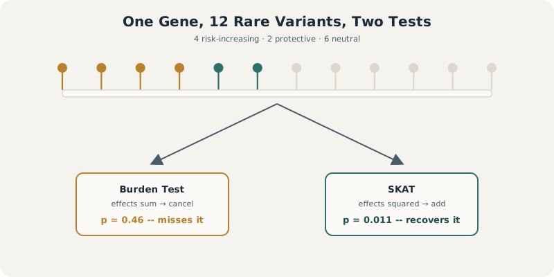
The tutorial’s central result in one picture: the same 12-variant gene, with the same causal architecture, gives two completely different answers depending on whether the test sums effects (burden) or sums their squares (SKAT).
SKATBurden TestRare VariantsR
Rare variants are, by definition, seen in only a handful of people. That single fact breaks almost every assumption a standard GWAS relies on, and it forces a completely different statistical toolkit.
This tutorial builds that toolkit from the ground up. We start with why single-variant testing fails, work through burden tests and SKAT by deriving their score statistics by hand, and finish with the saddlepoint approximation that makes rare-variant testing usable at biobank scale. Every statistic below is implemented in base R and checked against either a built-in R function or a Monte Carlo simulation.
1 Why Single-Variant Tests Fail for Rare Variants
If GWAS works for common variants, why not just run the same test on rare ones? Because you’ll rarely even observe the variant. A single-variant test needs carriers in your sample before it can say anything at all.
Large-effect variants on protein function are disproportionately rare, because natural selection removes them from the population before they become common. This is the central reason rare variants matter: the alleles most likely to have a real, interpretable effect on a trait are exactly the ones a standard genotyping array will barely capture.
The scale of the problem is easiest to see through a simple question: how many people do you need before you’re likely to observe even one carrier?
1.1 1.1 How many samples until you see one copy?
Assume random mating, so the two chromosomes carried by each of \(N\) individuals are independent draws with minor allele frequency \(p\). The probability of seeing zero copies of the variant is \((1-p)^{2N}\), so:
\[
P(\text{at least one copy}) = 1 - (1-p)^{2N} > 0.999 \quad\Longrightarrow\quad N > \frac{\log(0.001)}{2\log(1-p)}
\]
# Sample size needed to observe >= 1 copy of a variant with 99.9% probabilitymaf <-c(0.1, 0.01, 0.001, 0.0001)required_n <-log(0.001) / (2*log(1- maf))data.frame(MAF = maf, Required_N =ceiling(required_n))
A data.frame: 4 × 2
MAF
Required_N
<dbl>
<dbl>
1e-01
33
1e-02
344
1e-03
3453
1e-04
34538
Going from a MAF of 1% to 0.01% multiplies the required sample size a hundredfold. Single-variant testing simply runs out of carriers long before it runs out of interesting biology. And yet rare variants are collectively far from rare: each person carries roughly 200 rare coding variants, so a gene-level view of these variants is both necessary and has plenty of signal to work with.
2 Collapsing Variants Into a Gene-Level Burden
If no single variant has enough carriers, what do we test instead? We stop asking about one variant and start asking about a gene. Define a carrier as anyone with at least one rare variant in the region, and test whether carriers and non-carriers differ in disease risk.
This converts a sparse, high-dimensional problem (many rare variants, few carriers each) into a simple 2x2 question: are carriers more likely to be cases than non-carriers?
# A toy burden contingency table: carriers of a rare-variant burden vs disease statusburden_table <-matrix(c(14, 6, 5, 15), nrow =2, byrow =TRUE,dimnames =list(Status =c("Case", "Control"),Burden =c("Carrier", "Non-carrier")))burden_tablefisher.test(burden_table)
A matrix: 2 × 2 of type dbl
Carrier
Non-carrier
Case
14
6
Control
5
15
    Fisher's Exact Test for Count Data

data:  burden_table
p-value = 0.01039
alternative hypothesis: true odds ratio is not equal to 1
95 percent confidence interval:
  1.457116 35.737819
sample estimates:
odds ratio
  6.614723
The odds ratio of association follows directly from the table:
\[
\text{OR} = \frac{a/c}{b/d} = \frac{ad}{bc}
\]
With small carrier counts, a chi-squared test is unreliable, so fisher.test reaches for the exact hypergeometric distribution instead of a large-sample approximation. It’s worth confirming exactly what that function is computing.
3 Fisher’s Exact Test, From First Principles
What is fisher.test actually computing under the hood? The exact probability of observing a table at least as extreme as yours, conditional on the row and column totals staying fixed, under the hypergeometric distribution.
For a 2x2 table with cell counts \(a, b, c, d\), the probability of the observed table conditional on its margins is:
\[
P = \frac{\binom{a+b}{a}\binom{c+d}{c}}{\binom{n}{a+c}}
\]
The two-sided p-value sums this probability over every table with the same margins that is at least as unlikely as the one observed — not just the fraction for the observed table alone.
# Verify the hypergeometric formula by hand against R's Fisher testa <-14; b <-6; c <-5; d <-15row1 <- a + b; row2 <- c + dcol1 <- a + c; col2 <- b + dtotal <- row1 + row2p_observed <-choose(row1, a) *choose(row2, c) /choose(total, col1)cat("P(observed table) =", p_observed, "\n")possible_a <-max(0, col1 - row2):min(row1, col1)probs <-sapply(possible_a, function(x) {choose(row1, x) *choose(row2, col1 - x) /choose(total, col1)})p_two_sided <-sum(probs[probs <= p_observed +1e-8])cat("Two-sided p-value (by hand) =", p_two_sided, "\n")
0.0104 matches R’s reported 0.01039 to rounding. This is a useful sanity check to run once: it confirms fisher.test isn’t summing probabilities for tables that happen to be less extreme in only one direction, a mistake that’s easy to make when re-implementing exact tests by hand.
R.A. Fisher, who introduced this test alongside the concept of the null hypothesis, was explicit that a null hypothesis can only ever be rejected by data, never confirmed by it — a framing worth keeping in mind for every p-value that follows.
A single 2x2 table is a fine illustration, but it throws away information: every rare variant gets collapsed into one indicator, regardless of how rare it individually is, and regardless of whether its effect on the trait is protective or damaging. A regression framework fixes both problems.
4 A Regression Framework for Burden Testing
For a continuous trait, the natural model regresses the phenotype on every rare variant in the region:
Why weight variants at all, rather than just summing raw genotype counts? Because not every rare variant is equally rare. A weighting scheme that upweights rarer variants reflects the prior belief that rarer variants are more likely to be under stronger negative selection, and therefore more likely to matter.
A common choice, due to Wu et al. (2011), is \(w_j \sim \text{Beta}(\text{MAF}_j; 1, 25)\), which assigns steeply increasing weight as MAF approaches zero.
5 Simulating a Rare-Variant Test Gene
To make the rest of this tutorial concrete, we simulate a 12-variant gene in 4,000 individuals: four variants that increase disease risk, two that are protective, and six with no effect at all. This bidirectional architecture — some variants increase risk, others decrease it — is deliberately chosen, because it’s the setting where burden and variance-component tests are expected to behave differently.
set.seed(2026)n <-4000# sample sizeq <-12# number of rare variants in the genemaf <-runif(q, min =0.0005, max =0.01) # rare variant MAFs# Genotype matrix: 0/1/2 copies of the minor allele, drawn under Hardy-WeinbergG <-sapply(maf, function(p) rbinom(n, 2, p))colnames(G) <-paste0("v", seq_len(q))# One covariate (e.g. a normalized age term)X <-cbind(1, scale(rnorm(n)))colnames(X) <-c("Intercept", "Covariate")# Causal architecture: variants 1-4 increase risk, variants 5-6 are protective,# the remaining 6 are non-causal noise. Effects are deliberately bidirectional,# a setting where burden tests are known to lose power.true_beta <-c(1.3, 1.1, 1.0, 0.9, -1.4, -1.2, rep(0, q -6))alpha <-c(-2.2, 0.15) # covariate effects under the null model of disease risklinpred <- X %*% alpha + G %*% true_betapi_true <-1/ (1+exp(-linpred))y <-rbinom(n, 1, pi_true)cat("Cases:", sum(y), " Controls:", sum(y ==0), "\n")cat("MAFs:", round(maf, 4), "\n")saveRDS(list(G = G, X = X, y = y, maf = maf, true_beta = true_beta),"sim_data.rds")
A roughly 1:9 case-to-control ratio, which is typical of a moderately prevalent disease in a biobank cohort. This imbalance will matter a great deal later on.
With the gene simulated, we can now compute the Wu weight for each variant from its true MAF.
sim <-readRDS("sim_data.rds")maf <- sim$maf# Wu weights: w_j = Beta density of MAF under Beta(1, 25), upweighting rarer variantsw <-dbeta(maf, 1, 25)data.frame(variant =colnames(sim$G), MAF =round(maf, 4), weight =round(w, 2))
A data.frame: 12 × 3
variant
MAF
weight
<chr>
<dbl>
<dbl>
v1
0.0071
21.05
v2
0.0058
21.75
v3
0.0018
23.92
v4
0.0032
23.14
v5
0.0058
21.76
v6
0.0007
24.56
v7
0.0049
22.20
v8
0.0087
20.28
v9
0.0029
23.32
v10
0.0060
21.63
v11
0.0006
24.67
v12
0.0071
21.08
The rarest variant here (v11, MAF = 0.0006) gets almost 25% more weight than the most common one in the set (v8, MAF = 0.0087). This is a modest difference at these MAFs, but the gap widens sharply as MAF approaches the lower end of the exome-wide spectrum.
6 Three Classical Tests, and Why Genetics Prefers One of Them
Testing whether \(\beta_c \neq 0\) in a maximum-likelihood framework can be done three ways:
Wald test: fit the full (alternative) model, and measure how far the estimated effect is from zero, scaled by its standard error.
Likelihood ratio test (LRT): fit both the null and alternative models, and measure the drop in log-likelihood between them.
Score test: fit only the null model, and evaluate the gradient of the log-likelihood at that null.
All three measure the same underlying distance between the null hypothesis and the maximum-likelihood estimate, just along different geometric axes. As sample size grows, they converge to the same \(\chi^2_1\) distribution:
If they’re asymptotically the same, why does the choice matter for rare-variant testing? Computation. A modern biobank study tests tens of thousands of genes, often under a mixed model that corrects for relatedness and population structure. Fitting the full alternative model separately for every gene is computationally intractable. The score test only requires fitting the null model once — testing each gene afterward is just matrix multiplication against a fixed set of residuals.
This is the entire reason burden tests, SKAT, and SKAT-O are all built as score tests rather than Wald or LRT tests.
7 Deriving the Burden Score Statistic
Recall the weighted burden model, with burden score \(B_i = \sum_j w_j g_{i,j}\) for individual \(i\):
The \(\pi_i(1-\pi_i)\) terms cancel exactly, which is why the score function has such a clean form. Evaluated at the null (\(\beta_c = 0\), so \(\pi_i\) is replaced by its null-model prediction \(\hat\pi_i\)):
Intuitively: \(U(0)\) is large whenever people who carry more of the weighted burden also have larger-than-expected residuals — i.e., the gene’s cumulative dosage tracks disease status.
8 Testing the Burden Model in R
We fit the null model once (covariates only), compute residuals, and turn the derivation above directly into code.
sim <-readRDS("sim_data.rds")G <- sim$G; X <- sim$X; y <- sim$y; maf <- sim$mafw <-dbeta(maf, 1, 25)## --- Step 1: fit the null model (covariates only, no genotypes) ---null_model <-glm(y ~ X[, -1], family =binomial())pi_hat <-fitted(null_model)resid <- y - pi_hat## --- Step 2: build the weighted burden score B_i = sum_j w_j * G_ij ---B <-as.vector(G %*% w)## --- Step 3: burden score statistic U(0) = sum_i resid_i * B_i ---U0 <-sum(resid * B)## --- Step 4: variance of U(0) under the null ---## Var(U) = B' V B, where V = diag(pi_hat * (1 - pi_hat))V <- pi_hat * (1- pi_hat)var_U0 <-sum(V * B^2)## --- Step 5: score test statistic and p-value ---Q_burden <- U0^2/ var_U0p_burden_score <-pchisq(Q_burden, df =1, lower.tail =FALSE)cat("Burden score U(0) :", round(U0, 4), "\n")cat("Var[U(0)] :", round(var_U0, 4), "\n")cat("Burden score statistic :", round(Q_burden, 4), "\n")cat("Burden score p-value :", format.pval(p_burden_score, digits =4), "\n\n")## --- Compare to a Wald test from a direct logistic regression on the burden score ---alt_model <-glm(y ~ X[, -1] + B, family =binomial())wald_p <-summary(alt_model)$coefficients["B", "Pr(>|z|)"]cat("Wald test p-value (glm):", format.pval(wald_p, digits =4), "\n")
Two things stand out. First, the score and Wald p-values are close (0.46 and 0.44 land in the same non-significant territory), exactly the asymptotic equivalence discussed above. Second, and more importantly: the burden test completely misses this gene, despite it having six genuinely causal variants.
That’s not a bug in the implementation. It’s the burden test doing exactly what it’s designed to do, in a setting it’s poorly suited for.
9 When Burden Tests Fail: The Variance-Component Alternative
Why did the burden test fail here, specifically? Because four risk-increasing and two protective variants partially cancel out inside the same weighted sum. A burden test is only well-powered when all causal variants push risk in the same direction.
The naive fix — summing single-variant score statistics \(S_j = \sum_i g_{i,j}(y_i - \hat\pi_i)\) before squaring — has exactly this flaw:
\[
Q_B = \left(\sum_j w_j S_j\right)^2
\]
If variant A contributes \(S_A = +5\) and variant B contributes \(S_B = -5\), they cancel to zero and the association vanishes entirely, even though both variants are genuinely causal.
The fix, due to Wu et al. (2011) building on the C-alpha test of Neale et al. (2011), is to square each variant’s contribution before summing:
This is the SKAT (sequence kernel association test) statistic. Because residuals are squared before aggregation, risk-increasing and protective variants both contribute positively — nothing cancels.
10 Implementing SKAT From Scratch
\(Q_S\) is a quadratic form in the vector of per-variant score statistics, and under the null it follows a mixture of weighted \(\chi^2_1\) distributions rather than a single chi-squared distribution — one weight per eigenvalue of the statistic’s covariance kernel. We build that kernel directly, residualizing the genotype matrix on the covariates first, then get a p-value using the four-moment chi-squared approximation of Liu, Tang & Zhang (2009).
sim <-readRDS("sim_data.rds")G <- sim$G; X <- sim$X; y <- sim$y; maf <- sim$mafw <-dbeta(maf, 1, 25)## --- Null model (same as for the burden test) ---null_model <-glm(y ~ X[, -1], family =binomial())pi_hat <-fitted(null_model)resid <- y - pi_hatV <- pi_hat * (1- pi_hat)## --- Step 1: per-variant score statistics S_j = sum_i G_ij * resid_i ---S <-as.vector(t(G) %*% resid)## --- Step 2: SKAT statistic Q_S = sum_j w_j^2 * S_j^2 ---Q_skat <-sum(w^2* S^2)cat("SKAT statistic Q_S:", round(Q_skat, 3), "\n")## --- Step 3: null distribution of Q_S is a mixture of weighted chi-sq(1)'s.## Its "kernel" matrix comes from projecting G onto the space orthogonal to X## (so covariates are properly accounted for), then reweighting by w and V.Gt <- G - X %*%solve(t(X) %*% X) %*% (t(X) %*% G) # residualize G on XW <-diag(w)K <- W %*%t(Gt) %*%diag(V) %*% Gt %*% W # q x q kernel matrixlambda <-eigen(K, symmetric =TRUE, only.values =TRUE)$valueslambda <- lambda[lambda >1e-8]cat("Eigenvalues of the kernel matrix:", round(lambda, 2), "\n")## --- Step 4: Liu, Tang & Zhang (2009) moment-matching chi-square approximation ---liu_pvalue <-function(Q, lambda) { c1 <-sum(lambda) c2 <-sum(lambda^2) c3 <-sum(lambda^3) c4 <-sum(lambda^4) s1 <- c3 / c2^1.5 s2 <- c4 / c2^2if (s1^2> s2) { a <-1/ (s1 -sqrt(s1^2- s2)) delta <- s1 * a^3- a^2 df <- a^2-2* delta } else { a <-1/ s1 delta <-0 df <- c2^3/ c3^2 } muQ <- c1 sigmaQ <-sqrt(2* c2) muX <- df + delta sigmaX <-sqrt(2* (df +2* delta)) Qnorm <- (Q - muQ) / sigmaQ * sigmaX + muXpchisq(Qnorm, df = df, ncp = delta, lower.tail =FALSE)}p_skat <-liu_pvalue(Q_skat, lambda)cat("SKAT p-value (Liu et al. 2009 approximation):", format.pval(p_skat, digits =4), "\n")
SKAT statistic Q_S: 45891.8
Eigenvalues of the kernel matrix: 3155.72 2340.21 2230.61 1851.55 1809.8 1770.95 1683.92 1596.49 1357.32 865.01 511.66 502.97
SKAT p-value (Liu et al. 2009 approximation): 0.01069
SKAT recovers the association (p = 0.011) that the burden test missed entirely (p = 0.46), on the exact same data. This is the textbook case for variance-component tests: causal variants with mixed effect directions.
It’s worth checking this analytic p-value against a direct simulation, since the moment-matching approximation is, after all, an approximation.
sim <-readRDS("sim_data.rds")G <- sim$G; X <- sim$X; y <- sim$y; maf <- sim$mafw <-dbeta(maf, 1, 25)null_model <-glm(y ~ X[, -1], family =binomial())pi_hat <-fitted(null_model)V <- pi_hat * (1- pi_hat)Q_obs <- { resid <- y - pi_hat S <-as.vector(t(G) %*% resid)sum(w^2* S^2)}set.seed(1)B <-20000Q_null <-numeric(B)for (b inseq_len(B)) { y_perm <-rbinom(length(y), 1, pi_hat) # simulate under the fitted null resid_perm <- y_perm - pi_hat S_perm <-as.vector(t(G) %*% resid_perm) Q_null[b] <-sum(w^2* S_perm^2)}p_mc <-mean(Q_null >= Q_obs)cat("Monte Carlo p-value (", B, "null draws ):", p_mc, "\n")
Monte Carlo p-value ( 20000 null draws ): 0.01505
0.015 against the analytic 0.011: close enough to trust the moment-matching approximation for this gene, and a good habit to keep whenever a new test statistic goes into a pipeline.
11 SKAT-O: Combining Burden and Variance-Component Information
Neither test is uniformly better. Burden tests are more powerful when every causal variant pushes the trait in the same direction; SKAT is more powerful when effects are mixed or only a subset of variants are causal. SKAT-O (Lee et al., 2012) sidesteps the choice by taking a weighted combination of both statistics:
and searching over a grid of \(\rho\) values, with a correction for having tested several of them. \(\rho=0\) recovers pure SKAT; \(\rho=1\) recovers the pure burden test.
Minimum p-value across rho grid: 0.01069 at rho = 0
(SKAT-O then applies its own correction for testing multiple rho values;
  shown here to illustrate the interpolation, not as a calibrated final p-value.)
For this gene, \(\rho = 0\) (pure SKAT) is best, which is exactly what we’d expect given the bidirectional effect design. Note that this implementation illustrates the interpolation qualitatively rather than reproducing Lee et al.’s exact null distribution, which accounts for the correlation between the burden and SKAT statistics across the whole \(\rho\) grid through a more involved numerical integration.
12 Which Variants Go Into the Test?
A gene-based test is only as good as the variant set fed into it. In practice, variants are grouped by predicted functional consequence before testing:
Damaging missense: amino-acid-changing variants predicted deleterious by tools like CADD, PolyPhen, or SIFT
Synonymous: typically included as a negative control, since these shouldn’t affect protein function
Different genes show enrichment for different variant classes depending on their biology, so most modern rare-variant pipelines run several MAF cutoffs (e.g., <1%, <0.1%, <0.01%) crossed with several annotation categories for each gene, rather than committing to one variant set up front.
13 The Hidden Problem at Biobank Scale: Case-Control Imbalance
Everything above relies on the Central Limit Theorem: the null distribution of a score statistic is assumed to converge to a symmetric Normal. That assumption quietly depends on having enough carriers and a reasonably balanced number of cases and controls. Biobank-scale binary traits routinely have neither.
We can see this directly by simulating the null distribution of a single-variant score statistic under three regimes.
The common-variant and rare-but-balanced cases match the Normal approximation closely, exactly as CLT theory promises. The rare-and-imbalanced case is a different story: skewness jumps to 1.29, and the true tail probability is nearly 18-fold larger than the Normal approximation would suggest.
That’s not a small correction. At genome-wide or exome-wide significance thresholds (typically \(5\times10^{-8}\) or stricter after multiple testing correction), an 18-fold underestimate of the p-value in the tail translates directly into false positives.
14 The Saddlepoint Approximation: Fixing the Tail
If the Normal approximation only uses the mean and variance, what would a better approximation use? Every moment of the distribution, via its cumulant generating function (CGF), and — critically — it approximates the distribution at the specific point in the tail you care about, rather than at the center.
The CGF is the log of the moment generating function, \(K(t) = \log \mathbb{E}[e^{tX}]\). Its derivatives at \(t=0\) recover the ordinary moments (variance, skewness, kurtosis), but its real advantage is computational: because our score statistic is a sum of independent per-individual contributions, \(K(t)\) for the total is just the sum of each individual’s CGF, whereas the moment generating functions would need to be multiplied — a much less numerically stable operation once you’re summing thousands of terms.
The saddlepoint approximation (SPA) uses the full CGF to re-center the approximation exactly at the observed test statistic, rather than at the mean. It solves for a ‘tilting’ parameter \(\hat t\) satisfying \(K'(\hat t) = q_{\text{obs}}\), then uses the curvature of \(K\) at that point to get an accurate tail probability — the Lugannani-Rice formula. This is the method behind SAIGE-GENE+’s improved type-I error control at rare, imbalanced traits.
set.seed(7)n <-5000maf <-0.005case_rate <-0.01pi_hat <-rep(case_rate, n)g <-rbinom(n, 2, maf)sigma <-sqrt(sum(pi_hat * (1- pi_hat) * g^2))## CGF of a single term X_i = g_i * (Y_i - pi_i), Y_i ~ Bernoulli(pi_i)K_i <-function(t, g_i, p_i) log((1- p_i) *exp(-t * g_i * p_i) + p_i *exp(t * g_i * (1- p_i)))K1_i <-function(t, g_i, p_i) { h <-1e-5; (K_i(t + h, g_i, p_i) -K_i(t - h, g_i, p_i)) / (2* h) }K2_i <-function(t, g_i, p_i) { h <-1e-4; (K_i(t + h, g_i, p_i) -2*K_i(t, g_i, p_i) +K_i(t - h, g_i, p_i)) / h^2 }K_total <-function(t) sum(sapply(seq_len(n), function(i) K_i(t, g[i], pi_hat[i])))K1_total <-function(t) sum(sapply(seq_len(n), function(i) K1_i(t, g[i], pi_hat[i])))K2_total <-function(t) sum(sapply(seq_len(n), function(i) K2_i(t, g[i], pi_hat[i])))## Test statistic set at 3 standard deviations - the "borderline significant" regionq_obs <-3* sigmacat("sigma =", round(sigma, 3), " q_obs (3 sd) =", round(q_obs, 3), "\n")## Solve the saddlepoint equation K'(t_hat) = q_obsthat <-uniroot(function(t) K1_total(t) - q_obs, interval =c(1e-6, 5))$root## Lugannani-Rice saddlepoint approximation for P(S >= q_obs)w <-sign(that) *sqrt(2* (that * q_obs -K_total(that)))u <- that *sqrt(K2_total(that))p_spa <-pnorm(w, lower.tail =FALSE) +dnorm(w) * (1/ u -1/ w)## Compare to the naive Normal approximation using only mean & variancep_normal <-pnorm(q_obs, mean =0, sd = sigma, lower.tail =FALSE)## Monte Carlo "ground truth"B <-2000000mc_scores <-replicate(B, sum(g * (rbinom(n, 1, pi_hat) - pi_hat)))p_mc <-mean(mc_scores >= q_obs)cat("Saddlepoint t_hat :", round(that, 4), "\n")cat("SPA p-value :", format.pval(p_spa, digits =4), "\n")cat("Normal-approx p-value :", format.pval(p_normal, digits =4), "\n")cat("Monte Carlo p-value :", format.pval(p_mc, digits =4), "(", B, "draws )\n")
sigma = 0.704  q_obs (3 sd) = 2.111
Saddlepoint t_hat        : 1.6964
SPA p-value              : 0.01289
Normal-approx p-value    : 0.00135
Monte Carlo p-value      : 0.01394 ( 2e+06 draws )
The saddlepoint approximation (0.0129) tracks the 2-million-draw Monte Carlo truth (0.0139) closely. The Normal approximation (0.00135), by contrast, is off by roughly an order of magnitude at exactly the same test statistic. This single comparison is the entire justification for why SAIGE-GENE+, and every serious modern rare-variant tool, replaces the Normal approximation with SPA before reporting a p-value.
15 Choosing a Method in Practice
No single test is correct for every study design. The right choice depends on relatedness structure, sample size, trait type, and case-control balance.
As a rule of thumb: the more imbalanced or related your samples, the more you need a method built around a mixed model with saddlepoint-corrected p-values, rather than a method that assumes independence and a Normal null.
16 Summary
Rare variants are individually hard to detect, but collectively common enough to test as a group.
Burden tests and SKAT differ in one key assumption: whether causal effects within a gene point in the same direction.
Both are implemented as score tests specifically because biobank-scale analysis makes fitting the full alternative model, gene by gene, computationally infeasible.
SKAT-O interpolates between burden and SKAT rather than forcing a choice between them.
At rare variant frequencies and with case-control imbalance, the Normal approximation that score tests rely on breaks down badly — the saddlepoint approximation is what makes modern tools like SAIGE-GENE+ trustworthy at genome-wide significance thresholds.
17 References
Foundational methods
Li, B. & Leal, S. M. (2008). Methods for detecting associations with rare variants for common diseases: application to analysis of sequence data. American Journal of Human Genetics, 83, 311–321.
Madsen, B. E. & Browning, S. R. (2009). A groupwise association test for rare mutations using a weighted sum statistic. PLoS Genetics, 5, e1000384.
Price, A. L. et al. (2010). Pooled association tests for rare variants in exon-resequencing studies. American Journal of Human Genetics, 86, 832–838.
Neale, B. M. et al. (2011). Testing for an unusual distribution of rare variants. PLoS Genetics, 7, e1001322.
Wu, M. C. et al. (2011). Rare-variant association testing for sequencing data with the sequence kernel association test. American Journal of Human Genetics, 89, 82–93.
Lee, S., Wu, M. C. & Lin, X. (2012). Optimal tests for rare variant effects in sequencing association studies. Biostatistics, 13, 762–775.
Lee, S. et al. (2012). Optimal unified approach for rare-variant association testing with application to small-sample case-control whole-exome sequencing studies. American Journal of Human Genetics, 91, 224–237.
Liu, H., Tang, Y. & Zhang, H. H. (2009). A new chi-square approximation to the distribution of non-negative definite quadratic forms in non-central normal variables. Computational Statistics & Data Analysis, 53, 853–856.
Scalable software and applications
Zhou, W. et al. (2020). Scalable generalized linear mixed model for region-based association tests in large biobanks and cohorts. Nature Genetics, 52, 634–639.
Zhou, W., Bi, W., Zhao, Z. et al. (2022). SAIGE-GENE+ improves the efficiency and accuracy of set-based rare variant association tests. Nature Genetics, 54, 1466–1469.
Backman, J. D. et al. (2021). Exome sequencing and analysis of 454,787 UK Biobank participants. Nature, 599, 628–634.
Karczewski, K. J. et al. (2022). Systematic single-variant and gene-based association testing of thousands of phenotypes in 394,841 UK Biobank exomes. Cell Genomics, 2, 100168.