t-test or ANOVA? Choosing the Right Test for Before/After Treatment Across Multiple Groups
Why ‘before vs. after’ and ‘how many groups’ are two separate questions
Author
Nivedita
Published
August 4, 2026
1 Introduction
A question that comes up constantly in applied statistics: there are several groups — say, three treatment arms — and each subject is measured before and after treatment. Should the comparison use a t-test or an ANOVA?
This question, as posed, is missing information. The correct test depends on two things simultaneously: the number of groups, and the number of time points measured within each subject. Misjudging either one produces a test that is underpowered, statistically invalid, or answering a different question than the one intended.
This tutorial develops the decision logic, demonstrates why naive approaches fail, and works through a complete example using a mixed-design (repeated-measures) ANOVA — the test that fits a multi-group before/after design.
2 What a t-test Can and Cannot Test
A t-test compares two means. Two variants are relevant to this design.
An independent-samples t-test compares two separate groups measured once each — for example, a treatment group versus a control group, both assessed after treatment. The two sets of observations arise from different subjects.
A paired t-test compares two measurements taken from the same subjects — for example, a biomarker measured before and after treatment within a single group. Pairing removes between-subject variability from the comparison, which increases statistical power relative to treating the two measurements as independent.
Q: Why can’t a single t-test handle a multi-group before/after design directly? A: Each t-test variant models exactly one source of variation — either differences between groups or differences between time points — but not both together. A before/after study with three treatment arms contains both sources of variation at once, and neither t-test variant has a mechanism for modeling their combination.
3 Why Not Run Several t-tests?
A common workaround is to run a paired t-test separately within each group, or an independent t-test at each time point, and compare the pattern of results informally. This approach fails for two reasons.
First, running multiple significance tests on related data inflates the family-wise Type I error rate, since each additional test carries its own probability of a false positive. With three groups tested separately, the effective error rate across the family of tests exceeds the nominal 0.05 threshold intended for a single test.
Second, and more fundamentally, separate t-tests cannot test the question a multi-group before/after design is built to answer: did the treatment effect — the before-to-after change — differ across groups? A set of individual paired t-tests indicates whether each group changed on its own, but provides no formal test of whether the magnitude of change differed between groups. That comparison is the group × time interaction, and testing it requires a model that includes both factors jointly.
4 The Mixed-Design ANOVA
A mixed-design ANOVA (also termed a between-within ANOVA) models two factors simultaneously:
Time (or condition) is a within-subjects factor: before and after values come from the same subjects and are therefore correlated.
Group is a between-subjects factor: treatment arms consist of different, independent subjects.
The model partitions variance into three components: a main effect of time (whether values changed overall), a main effect of group (whether groups differ overall), and a group × time interaction (whether the magnitude of change depended on group membership).
Q: Which of these three effects answers the original research question? A: In a treatment-comparison study, the interaction term is typically the effect of interest. A significant interaction indicates that groups did not all change by the same amount, which is the statistical signature of a treatment effect that differs from whatever change occurred in the comparison arms.
5 Decision Guide
Design
Test
Two groups, one time point
Independent-samples t-test
One group, two time points
Paired t-test
Two groups, two time points (before/after)
Mixed ANOVA, or a t-test on change scores
More than two groups, two time points
Mixed ANOVA
More than two time points, with or without multiple groups
Repeated-measures or mixed ANOVA
6 Worked Example: A Biomarker Across Three Groups
Consider three groups — A, B, and C — with a biomarker recorded for each subject under two conditions: control and treatment. This is a 3 × 2 mixed design: group is between-subjects, condition is within-subjects, since each subject contributes both a control and a treatment value.
The simulation below generates 15 subjects per group, with the treatment effect itself set to differ by group: group A shows a minimal response, group B a moderate response, and group C a strong response. This is the pattern a mixed ANOVA is designed to detect via the group × condition interaction.
set.seed(42)n_per_group <-15# subjects per group# Simulate a biomarker with a group-specific baseline and a group-specific# treatment response (this is what creates a group x condition interaction)simulate_group <-function(group_id, baseline, effect) { subject <-paste0(group_id, "_", seq_len(n_per_group)) control <-rnorm(n_per_group, mean = baseline, sd =5) treatment <- control +rnorm(n_per_group, mean = effect, sd =3)data.frame(subject =rep(subject, 2),group = group_id,condition =rep(c("control", "treatment"), each = n_per_group),biomarker =c(control, treatment) )}df <-rbind(simulate_group("A", baseline =50, effect =2), # minimal responsesimulate_group("B", baseline =50, effect =8), # moderate responsesimulate_group("C", baseline =50, effect =15) # strong response)df$group <-factor(df$group)df$condition <-factor(df$condition, levels =c("control", "treatment"))df$subject <-factor(df$subject)head(df, 6)
A data.frame: 6 × 4
subject
group
condition
biomarker
<fct>
<fct>
<fct>
<dbl>
1
A_1
A
control
56.85479
2
A_2
A
control
47.17651
3
A_3
A
control
51.81564
4
A_4
A
control
53.16431
5
A_5
A
control
52.02134
6
A_6
A
control
49.46938
aggregate(biomarker ~ group + condition, data = df, mean)
A data.frame: 6 × 3
group
condition
biomarker
<fct>
<fct>
<dbl>
A
control
52.42117
B
control
48.28969
C
control
51.12821
A
treatment
53.37999
B
treatment
56.58443
C
treatment
66.59590
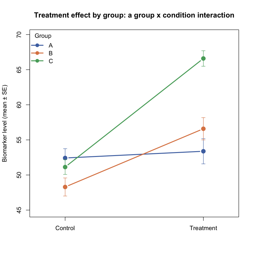
Group A moves from approximately 52.4 to 53.4 (a minimal shift), group B moves from approximately 48.3 to 56.6, and group C moves from approximately 51.1 to 66.6. The response grows across groups, as specified in the simulation.
# Mixed ANOVA: condition is within-subjects (each subject has a control AND# a treatment value), group is between-subjects. Error(subject/condition)# tells R that condition is nested within subject.model <-aov(biomarker ~ group * condition +Error(subject / condition), data = df)summary(model)
Error: subject
          Df Sum Sq Mean Sq F value  Pr(>F)
group      2  770.3   385.2   7.431 0.00173 **
Residuals 42 2177.0    51.8
---
Signif. codes:  0 ‘***’ 0.001 ‘**’ 0.01 ‘*’ 0.05 ‘.’ 0.1 ‘ ’ 1

Error: subject:condition
                Df Sum Sq Mean Sq F value   Pr(>F)
condition        1 1527.8  1527.8  279.79  < 2e-16 ***
group:condition  2  789.4   394.7   72.28 2.52e-14 ***
Residuals       42  229.4     5.5
---
Signif. codes:  0 ‘***’ 0.001 ‘**’ 0.01 ‘*’ 0.05 ‘.’ 0.1 ‘ ’ 1
The output contains two error strata, corresponding to the between-subjects and within-subjects portions of the design.
The subject stratum tests the main effect of group (\(p = 0.00173\)): the three groups differ overall, averaging control and treatment together.
The subject:condition stratum tests the main effect of condition (\(p < 2\mathrm{e}{-16}\)) and, critically, the group × condition interaction (\(p = 2.52\mathrm{e}{-14}\)).
Q: Which result answers the original question — did treatment work differently by group? A: The interaction term. Its significance indicates that the magnitude of the control-to-treatment change is not the same across groups A, B, and C. A significant main effect of condition alone would only indicate that biomarker levels changed on average; the interaction indicates that the treatment effect itself depends on group membership. Three separate paired t-tests, one per group, would indicate whether each group changed individually, but would provide no formal test of whether those three changes differed from one another — which is ordinarily the scientific question of interest in a treatment-comparison study.
The table of F-statistics makes the interaction’s significance clear, but doesn’t show what that interaction actually looks like. The plot below does: each line traces one group’s mean biomarker level from control to treatment, with error bars showing the standard error of the mean. A mixed ANOVA with no interaction would produce three roughly parallel lines — all groups shifting by about the same amount. What the simulation shows instead is divergence: group C’s line rises steeply, group B’s rises more modestly, and group A’s is nearly flat.
# Group means and standard errors by condition, for the interaction plotsummary_df <-aggregate(biomarker ~ group + condition, data = df,FUN =function(x) c(mean =mean(x), se =sd(x) /sqrt(length(x))))summary_df <-do.call(data.frame, summary_df)names(summary_df) <-c("group", "condition", "mean", "se")summary_df
A data.frame: 6 × 4
group
condition
mean
se
<fct>
<fct>
<dbl>
<dbl>
A
control
52.42117
1.323583
B
control
48.28969
1.286907
C
control
51.12821
1.045192
A
treatment
53.37999
1.793629
B
treatment
56.58443
1.587070
C
treatment
66.59590
1.105771
group_colors <-c(A ="#4C72B0", B ="#DD8452", C ="#55A868")plot(NULL, xlim =c(0.8, 2.2),ylim =range(c(summary_df$mean - summary_df$se, summary_df$mean + summary_df$se)) +c(-2, 2),xaxt ="n", xlab ="", ylab ="Biomarker level (mean \u00B1 SE)",main ="Treatment effect by group: a group x condition interaction")axis(1, at =c(1, 2), labels =c("Control", "Treatment"))for (g inlevels(summary_df$group)) { sub <- summary_df[summary_df$group == g, ] sub <- sub[order(sub$condition), ] x <-c(1, 2)lines(x, sub$mean, col = group_colors[g], lwd =2.5, type ="b", pch =19, cex =1.3)arrows(x, sub$mean - sub$se, x, sub$mean + sub$se, angle =90, code =3,length =0.05, col = group_colors[g])}legend("topleft", legend =levels(summary_df$group), col = group_colors, lwd =2.5, pch =19,title ="Group", bty ="n")
Non-parallel lines are the visual signature of an interaction — and the degree of non-parallelism here (group C pulling sharply away from A and B) is exactly what produced the very small p-value on the group:condition term above. This plot and the ANOVA table are two views of the same result: one gives the formal test, the other shows what the tested pattern actually looks like in the data, which is often the more persuasive figure for a paper or presentation.
7 Assumptions and Alternatives
The mixed-design ANOVA carries the standard ANOVA assumptions of normally distributed residuals and homogeneity of variance across groups, together with sphericity for the within-subjects factor when more than two time points are present. Sphericity is automatically satisfied with only two levels, as in a single before/after comparison.
Where these assumptions are doubtful, two alternatives are available. A linear mixed-effects model, fit with lme4 or nlme, accommodates unbalanced data and missing observations more gracefully than classical ANOVA while producing an equivalent interaction test. For small samples or markedly non-normal outcomes, a nonparametric alternative such as the Friedman test, combined with rank-based group comparisons, can be used, though these approaches test somewhat different hypotheses and offer less flexibility for interaction effects.
8 Conclusion
“t-test or ANOVA” is not, by itself, a well-posed question. The determining factor is the number of independent sources of variation present in the design. A before/after comparison within a single group constitutes one factor; a comparison across multiple groups introduces a second. When both are present together, as in a multi-group treatment study, the appropriate test is one built to model two factors and their interaction jointly — the mixed-design ANOVA. Substituting a t-test in this setting does not merely reduce statistical power; it silently discards the interaction test that the design was intended to answer.