Twins, Variance, and the Logic of Heritability

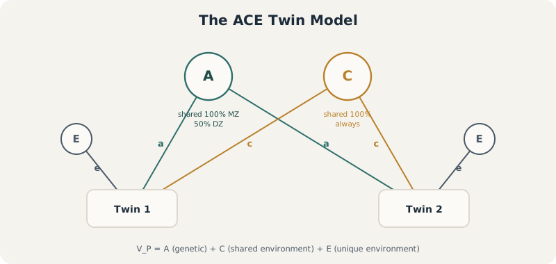
How ACE models turn twin correlations into estimates of nature and nurture

Why MZ and DZ twins let us split trait variance into genetic and environmental pieces – from Falconer’s back-of-envelope formula to a fitted ACE model to SNP-based heritability in unrelated people.

The one fact this whole tutorial runs on: MZ and DZ twins share C and E equally, but differ in exactly how much of A they share – which is enough, on its own, to separate genetic from environmental variance.

Heritability ACE Model Twin Studies R

Why do some siblings look and behave almost identically, while others in the same family seem to have little in common?

Height, cognitive ability, disease risk — nearly every measurable human trait varies from person to person.

How much of that variation comes from genetic differences, and how much comes from the environment people happen to grow up in?

That question is what heritability tries to answer. This tutorial builds the idea up from scratch: what heritability actually means, why twins are uniquely suited to estimate it, how that logic becomes a fitted statistical model, and how the same idea extends beyond twins to unrelated people using DNA directly.

1 Heritability Is a Statement About Variance, Not About You

A heritability of 70% does not mean 70% of your height is genetic.

Heritability describes how much of the variation across a population is attributable to genetic differences. It says nothing about any one individual.

Phenotypic variance splits into two pieces:

\[V_P = V_G + V_E\]

where \(V_P\) is the total observed variance in a trait, \(V_G\) is the share attributable to genetic differences between people, and \(V_E\) is the share attributable to environmental differences.

Heritability is simply the genetic fraction of that total:

\[h^2 = \frac{V_G}{V_P}, \qquad 0 \le h^2 \le 1\]

A trait can be highly heritable and still change dramatically across generations. Human height sits around \(h^2 \approx 0.8\), yet average height rose substantially over the 20th century as nutrition and healthcare improved. High heritability describes current variance, not future immutability — and it is specific to the population it was measured in. A population with little environmental variation will show a higher \(h^2\) than one with large environmental disparities, for the exact same trait and the exact same genetics, simply because \(V_E\) differs between them.

2 Why Twins Are a Natural Experiment

Directly separating \(V_G\) from \(V_E\) in an ordinary sample is impossible — you never observe the same person raised in two different genetic or environmental worlds.

Twins offer a workaround, because two twin types differ in exactly one respect.

Monozygotic (MZ) twins  →  share ~100% of their segregating genetic variants
Dizygotic (DZ) twins    →  share ~50% of their segregating genetic variants, on average

Both twin types, raised together, are assumed to share their rearing environment equally.

If a trait is influenced by genetics, MZ twins — who share all their genes — should resemble each other more closely than DZ twins, who share only half. The size of that gap between MZ and DZ similarity is where an estimate of heritability comes from.

3 From Twin Correlations to Variance Components

Twin models split phenotypic variance into three parts rather than two:

\[V_P = A + C + E\]

A  =  additive genetic variance        (variants add up across the genome)
C  =  shared (common) environment      (identical for both twins in a pair)
E   =  unique environment               (everything that differs within a pair,
                                          including measurement error)

Given the sharing rules above, the expected correlation between twins works out to:

\[r_{MZ} = A + C\] \[r_{DZ} = \tfrac{1}{2}A + C\]

(All variances here are on the standardized scale, so \(A + C + E = 1\).)

Two equations, two unknowns — the difference between them isolates \(A\) directly.

4 Falconer’s Method

Subtracting the two correlation equations gives a strikingly simple estimator, due to Falconer (1960):

\[\hat{A} = 2(r_{MZ} - r_{DZ})\] \[\hat{C} = r_{MZ} - \hat{A}\] \[\hat{E} = 1 - r_{MZ}\]

No model-fitting software required — just two correlations and arithmetic. Let’s simulate twin data with known true variance components and check whether this recovers them.

simulate_twins <- function(n, a, c, e, shared_genetic_fraction) {
  # a, c, e are given as SDs; shared_genetic_fraction = 1 for MZ, 0.5 for DZ
  A_shared  <- rnorm(n, 0, a)
  A1_unique <- rnorm(n, 0, a * sqrt(1 - shared_genetic_fraction))
  A2_unique <- rnorm(n, 0, a * sqrt(1 - shared_genetic_fraction))
  A1 <- sqrt(shared_genetic_fraction) * A_shared + A1_unique
  A2 <- sqrt(shared_genetic_fraction) * A_shared + A2_unique

  C_shared <- rnorm(n, 0, c)
  E1 <- rnorm(n, 0, e)
  E2 <- rnorm(n, 0, e)

  data.frame(twin1 = A1 + C_shared + E1, twin2 = A2 + C_shared + E2)
}

set.seed(1)
n_pairs <- 2000
a2_true <- 0.50; c2_true <- 0.20; e2_true <- 0.30    # must sum to 1
a <- sqrt(a2_true); c <- sqrt(c2_true); e <- sqrt(e2_true)

mz <- simulate_twins(n_pairs, a, c, e, shared_genetic_fraction = 1.0)
dz <- simulate_twins(n_pairs, a, c, e, shared_genetic_fraction = 0.5)

r_mz <- cor(mz$twin1, mz$twin2)
r_dz <- cor(dz$twin1, dz$twin2)

cat(sprintf("MZ correlation: %.3f\n", r_mz))
cat(sprintf("DZ correlation: %.3f\n", r_dz))

MZ correlation: 0.708
DZ correlation: 0.439

h2_falconer <- 2 * (r_mz - r_dz)
c2_falconer <- r_mz - h2_falconer
e2_falconer <- 1 - r_mz

data.frame(
  component = c("A (genetic)", "C (shared env)", "E (unique env)"),
  true_value = c(a2_true, c2_true, e2_true),
  falconer_estimate = round(c(h2_falconer, c2_falconer, e2_falconer), 3)
)

A data.frame: 3 × 3

component	true_value	falconer_estimate
<chr>	<dbl>	<dbl>
A (genetic)	0.5	0.538
C (shared env)	0.2	0.170
E (unique env)	0.3	0.292

Falconer’s arithmetic recovers all three true values closely, using nothing more than two correlations.

That simplicity is also its ceiling. Falconer’s method gives no standard errors, no way to test whether \(C\) is actually needed at all, and no way to compare competing models formally. For that, twin research moved to full likelihood-based modeling — the same logic, expressed as a fitted statistical model instead of a shortcut formula.

5 Why Move to a Fitted Model?

Falconer’s estimator is a fixed, one-shot calculation. A structural equation model (SEM) treats \(A\), \(C\), and \(E\) as parameters to be estimated by maximum likelihood, given the raw twin data and the covariance structure implied by MZ/DZ sharing:

\[\Sigma_{MZ} = \begin{pmatrix} 1 & A + C \\ A + C & 1 \end{pmatrix}, \qquad \Sigma_{DZ} = \begin{pmatrix} 1 & \tfrac{1}{2}A + C \\ \tfrac{1}{2}A + C & 1 \end{pmatrix}\]

Fitting these by likelihood, rather than reading them off two correlations, buys three things at once: standard errors on \(A\), \(C\), and \(E\); the ability to constrain \(C=0\) or \(A=0\) and formally test whether that constrained model fits significantly worse; and a natural way to add covariates or handle missing data. This is exactly what dedicated twin-modeling software like OpenMx does under the hood — the version below implements the same likelihood directly, so the mechanics stay visible.

# Bivariate normal log-likelihood for a set of twin pairs, given a 2x2 covariance matrix (mean 0)
biv_normal_loglik <- function(dat, Sigma) {
  n <- nrow(dat)
  detS <- Sigma[1,1]*Sigma[2,2] - Sigma[1,2]^2
  Sinv <- matrix(c(Sigma[2,2], -Sigma[1,2], -Sigma[1,2], Sigma[1,1]), 2, 2) / detS
  x <- as.matrix(dat)
  quad <- rowSums((x %*% Sinv) * x)
  -0.5 * n * log(detS) - 0.5 * sum(quad) - n * log(2*pi)
}

# Negative log-likelihood for the ACE model (and constrained sub-models)
neg_ll_ACE <- function(par, fix_c = NA, fix_a = NA) {
  a2 <- if (!is.na(fix_a)) fix_a else plogis(par[1])
  c2 <- if (!is.na(fix_c)) fix_c else plogis(par[2]) * (1 - a2)
  e2 <- 1 - a2 - c2
  if (e2 <= 0) return(1e10)

  Sigma_mz <- matrix(c(1, a2 + c2, a2 + c2, 1), 2, 2)
  Sigma_dz <- matrix(c(1, 0.5*a2 + c2, 0.5*a2 + c2, 1), 2, 2)

  -(biv_normal_loglik(mz, Sigma_mz) + biv_normal_loglik(dz, Sigma_dz))
}

5.1 Fitting ACE, AE, and CE

Three models, nested inside each other: the full ACE model, and two restricted versions that force one component to zero.

fit_ACE <- function() {
  opt <- optim(c(0, 0), neg_ll_ACE, method = "Nelder-Mead")
  a2 <- plogis(opt$par[1]); c2 <- plogis(opt$par[2]) * (1 - a2); e2 <- 1 - a2 - c2
  list(a2 = a2, c2 = c2, e2 = e2, negLL = opt$value, df = 3)
}

fit_AE <- function() {
  f <- function(par) neg_ll_ACE(c(par[1], -1e6), fix_c = 0)
  opt <- optim(0, f, method = "Brent", lower = -10, upper = 10)
  a2 <- plogis(opt$par[1]); e2 <- 1 - a2
  list(a2 = a2, c2 = 0, e2 = e2, negLL = opt$value, df = 2)
}

fit_CE <- function() {
  f <- function(par) neg_ll_ACE(c(-1e6, par[1]), fix_a = 0)
  opt <- optim(0, f, method = "Brent", lower = -10, upper = 10)
  c2 <- plogis(opt$par[1]); e2 <- 1 - c2
  list(a2 = 0, c2 = c2, e2 = e2, negLL = opt$value, df = 2)
}

ace <- fit_ACE(); ae <- fit_AE(); ce <- fit_CE()

data.frame(
  model = c("ACE", "AE", "CE"),
  a2 = round(c(ace$a2, ae$a2, ce$a2), 3),
  c2 = round(c(ace$c2, ae$c2, ce$c2), 3),
  e2 = round(c(ace$e2, ae$e2, ce$e2), 3),
  neg2LL = round(2 * c(ace$negLL, ae$negLL, ce$negLL), 1)
)

A data.frame: 3 × 5

model	a2	c2	e2	neg2LL
<chr>	<dbl>	<dbl>	<dbl>	<dbl>
ACE	0.508	0.190	0.301	20975.0
AE	0.709	0.000	0.291	21001.4
CE	0.000	0.574	0.426	21173.7

The full ACE fit lands almost exactly on the true simulated values (0.50 / 0.20 / 0.30) — maximum likelihood recovers the same answer Falconer’s shortcut did, as it should when the model is correctly specified.

Dropping \(C\) (the AE model) doesn’t just zero it out — the genetic component \(\hat A\) jumps up to absorb the shared-environment variance that’s no longer available to explain the resemblance between twins. That’s a useful diagnostic on its own: watch what happens to the other components when you force one to zero.

5.2 Is the Extra Complexity of ACE Actually Justified?

A likelihood ratio test answers this directly: is the improvement in fit from adding \(C\) back in bigger than you’d expect from noise alone?

lrt_stat <- 2 * ae$negLL - 2 * ace$negLL
lrt_df   <- ace$df - ae$df
lrt_p    <- 1 - pchisq(lrt_stat, lrt_df)

cat(sprintf("LRT comparing AE against full ACE: chi-sq = %.2f, df = %d, p = %.5f\n",
            lrt_stat, lrt_df, lrt_p))

aic <- c(ACE = 2*ace$negLL + 2*ace$df,
         AE  = 2*ae$negLL  + 2*ae$df,
         CE  = 2*ce$negLL  + 2*ce$df)
cat("\nAIC by model (lower is better):\n")
print(round(aic, 1))

LRT comparing AE against full ACE: chi-sq = 26.37, df = 1, p = 0.00000

AIC by model (lower is better):
    ACE      AE      CE 
20981.0 21005.4 21177.7 

Both diagnostics agree: forcing \(C\) to zero makes the model fit significantly worse, and AIC prefers the full ACE model over either restricted alternative. In a real analysis, this is exactly the workflow — fit the full model and each restriction, then let the likelihood ratio test and AIC decide which components the data actually support, rather than assuming a particular model in advance.

This is the concrete payoff of moving from Falconer’s formula to a fitted model: a formal, quantitative answer to “does shared environment matter here?” — not just a point estimate.

6 Beyond Twins: Heritability From Unrelated People

Twin models lean on a pair of fixed relatedness values — MZ pairs share (on average) all their genetic variance, DZ pairs share half. Modern genomics can go further: instead of assuming relatedness from pedigree structure, measure it directly from genotypes at hundreds of thousands of SNPs, for people who aren’t related at all.

The genetic relationship matrix (GRM) between two individuals \(i\) and \(j\), using standardized genotypes, is:

\[GRM_{ij} = \frac{1}{M}\sum_{k=1}^{M} \tilde{x}_{ik}\, \tilde{x}_{jk}\]

where \(M\) is the number of SNPs and \(\tilde x\) denotes a genotype standardized to mean 0 and variance 1. Full siblings average close to 0.5 here, just like the pedigree expectation for DZ twins — but now it’s measured, not assumed, and it varies continuously even among people with no known family relationship at all.

The Haseman–Elston regression (Haseman and Elston 1972) turns this into a heritability estimate with a beautifully simple idea:

Pairs of people who are more genetically similar should also be more phenotypically similar — in direct proportion to how related they are.

Regressing pairwise phenotypic similarity on GRM values, the slope of that line is an estimate of SNP heritability. This is the logic that underlies GREML and GCTA (Yang et al. 2010) applied at genome-wide scale — the toy version below applies it to a small simulated cohort of unrelated individuals.

set.seed(2)
n_ind <- 300
n_snps <- 2000
maf <- runif(n_snps, 0.05, 0.5)

genotypes <- sapply(maf, function(p) rbinom(n_ind, 2, p))
geno_std  <- scale(genotypes)                 # standardize each SNP column
GRM       <- (geno_std %*% t(geno_std)) / n_snps

h2_true <- 0.5
genetic_effect    <- rnorm(n_snps, 0, sqrt(h2_true / n_snps))
genetic_component  <- as.numeric(scale(geno_std %*% genetic_effect)) * sqrt(h2_true)
env_component      <- rnorm(n_ind, 0, sqrt(1 - h2_true))
phenotype          <- genetic_component + env_component

pheno_outer <- outer(phenotype, phenotype)
idx <- upper.tri(GRM)

he_fit <- lm(pheno_outer[idx] ~ GRM[idx])
round(coef(summary(he_fit)), 4)

A matrix: 2 × 4 of type dbl

	Estimate	Std. Error	t value	Pr(>|t|)
(Intercept)	-0.0008	0.0043	-0.1892	0.8499
GRM[idx]	0.6392	0.1922	3.3250	0.0009

The regression slope — the Haseman–Elston estimate of SNP heritability — lands in the right neighborhood of the true value of 0.5, estimated entirely from unrelated individuals and their genotypes, with no twins or known family structure anywhere in sight.

This is the same conceptual move that let human genetics scale heritability estimation from small twin registries to biobanks of hundreds of thousands of unrelated people (Yang et al. 2010) — replace an assumed relatedness value (0, 0.5, or 1, from pedigree structure) with a measured one (any value in between, from genotypes), and the same regression logic still applies.

7 Key Takeaways

• Heritability describes variance across a population, not a property of any one person, and it changes with the population’s environmental context.
• Twin designs work because MZ and DZ pairs differ in exactly one thing — how much genetic variance they share — while (by assumption) sharing their environment equally.
• Falconer’s method turns two correlations into estimates of A, C, and E with simple arithmetic, and recovers the truth well in simulation.
• A fitted SEM (the ACE model) reproduces Falconer’s estimates while adding what arithmetic alone can’t: standard errors, and formal likelihood ratio / AIC comparisons between nested models like ACE, AE, and CE.
• The same logic extends past twins entirely — the Haseman–Elston regression estimates heritability from measured genetic relatedness (a GRM) among people who share no known family relationship at all.

8 References

Falconer, D. S. (1960). Introduction to Quantitative Genetics. Oliver and Boyd.

Neale, M. C., & Cardon, L. R. (1992). Methodology for Genetic Studies of Twins and Families. Kluwer Academic Publishers.

Haseman, J. K., & Elston, R. C. (1972). The investigation of linkage between a quantitative trait and a marker locus. Behavior Genetics, 2(1), 3–19.

Yang, J., Benyamin, B., McEvoy, B. P., Gordon, S., Henders, A. K., Nyholt, D. R., Madden, P. A., Heath, A. C., Martin, N. G., Montgomery, G. W., Goddard, M. E., & Visscher, P. M. (2010). Common SNPs explain a large proportion of the heritability for human height. Nature Genetics, 42(7), 565–569.

Polderman, T. J. C., Benyamin, B., de Leeuw, C. A., Sullivan, P. F., van Bochoven, A., Visscher, P. M., & Posthuma, D. (2015). Meta-analysis of the heritability of human traits based on fifty years of twin studies. Nature Genetics, 47(7), 702–709.